Unit-3
Summarization Measures
Question bank
Part-A
Q1) Explain average and its significances. (5)
A1)
According to Professor Bowley, averages are “statistical constants which enable us to comprehend in a single effort the significance of the whole”. An average is a single value which is considered as the most representative for a given set of data. Measures of central tendency show the tendency of some central value around which data tend to cluster.
Significance of the Measure of Central Tendency
Measure of central tendency enables us to get a single value from the mass
Of data and also provide an idea about the entire data.
Measures of central tendency enable us to compare two or more than two populations by reducing the mass of data in one single figure. The comparison can be made either at the same time or over a period of time.
Q2) What are the properties of a good average? (7)
A2)
- Since we use the measures of central tendency to simplify the complexity of a data, so an average should be understandable easily otherwise its use is bound to be very limited.
- An average not only should be easy to understand but also should be simple to compute, so that it can be used as widely as possible.
3. A measure of central tendency should be defined properly so that it has an appropriate interpretation. It should also have an algebraic formula so that if different people compute the average from same figures, they get the same answer.
4. A measure of central tendency should be liable for the algebraic manipulations. If there are two sets of data and the individual information is available for both set, then one can be able to find the information regarding the combined set also then something is missing.
5. If any measure of central tendency is used to analyse the data, it is desirable that each and every observation is used for its calculation.
6. It is assumed that each and every observation influences the value of the average. If one or two very small or very large observations affect the average i.e. either increase or decrease its value largely, then the average cannot be consider as a good average.
Q3) Explain quartiles. (8)
A3)
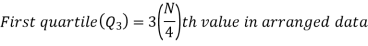
There are three quartiles, i.e. Q1, Q2 and Q3 which divide the total data into four equal parts when it has been orderly arranged. Q1, Q2 and Q3 are termed as first quartile, second quartile and third quartile or lower quartile, middle quartile and upper quartile, respectively. The first quartile, Q1, separates the first one-fourth of the data from the upper three fourths and is equal to the 25th percentile. The second quartile, Q2, divides the data into two equal parts (like median) and is equal to the 50th percentile. The third quartile, Q3, separates the first three-quarters of the data from the last quarter and is equal to 75th percentile.
For ungrouped data, we find the quartiles as follows-
For grouped data, we find the quartiles as follows-
i’th quartile can be find as-
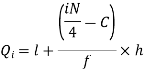
l = lower class limit of i'th quartile class,
h = width of the ith quartile class,
N = total frequency,
C = cumulative frequency of pre ith quartile class, and
f = frequencies of ith quartile class.
Q4) What is more than and less than ogive? (5)
A4)
Less Than Ogive: If we plot the points with the upper limits of the classes as abscissae and the cumulative frequencies corresponding to the values less then the upper limits as ordinates and join the points so plotted by line segments, the curve thus obtained is nothing but known as “less than cumulative frequency curve” or “less than ogive”.
More Than Ogive: If we plot the points with the lower limits of the classes as
Abscissae and the cumulative frequencies corresponding to the values more than the lower limits as ordinates and join the points so plotted by line segments, the curve thus obtained is nothing but known as “more than cumulative frequency curve” or “more than ogive”.
Q5) What is the significance of measures of dispersion? (5)
A5)
Measures of variation are pointed out as to how far an average is representative of the entire data. When variation is less, the average closely represents the individual values of the data and when variation is large; the average may not closely represent all the units and be quite unreliable.
Another purpose of measuring variation is to determine the nature and causes of variations in order to control the variation itself. Measurements of dispersion are helpful to control the causes of variation.
Many powerful statistical tools in statistics such as correlation analysis, the testing of hypothesis, the analysis of variance, techniques of quality control, etc. are based on different measures of dispersion.
Q6) Give the different formulae to calculate the SD. (8)
A6)
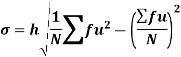
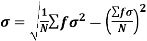
SD is defined as the positive square root of the arithmetic mean of the square of the deviation of the given values from their arithmetic mean. It is denoted by the symbol  .
.
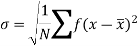
Where  is A.M of the distribution
  . We have more formulae to calculate the standard deviation.

 ….
…. 
In frequency distribution from, we put  where H is generally taken as width of class interval
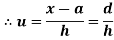
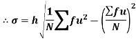
Shortcut formula to calculate standard deviation-
The square of the standard deviation is called known as a variance.

Q7) What are the advantages and disadvantages of variance? (7)
A7)
Advantages:
1. It is rigidly defined;
2. It utilizes all the observations;
3. Amenable to algebraic treatment;
4. Squaring is a better technique to get rid of negative deviations; and
5. It is the most popular measure of dispersion.
Disadvantages:
1. In cases where mean is not a suitable average, standard deviation may not be the coveted measure of dispersion like when open end classes are present. In such cases quartile deviation may be used;
2. It is not unit free;
3. Although easy to understand, calculation may require a calculator or a computer; and
4. Its unit is square of the unit of the variable due to which it is difficult to judge the magnitude of dispersion compared to standard deviation.
Q8) What is variance and variance of combined series? (7)
A8)
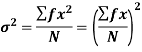
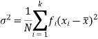
Variance is the average of the square of deviations of the values taken from mean. Taking a square of the deviation is a better technique to get rid of negative deviations.
Variance is given as-
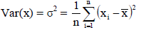
And for a frequency distribution, the formula is
Variance of the combined series-
If σ1, σ2 are two standard deviations of two series of sizes n1 and n2 with means ȳ1 and ȳ2. The variance of the two series of sizes n1 + n2 is:
σ 2 = (1/ n1 + n2) ÷ [n1 (σ1 2 + d1 2) + n2 (σ2 2 + d2 2)]
Where, d1 = ȳ 1 −ȳ , d2 = ȳ 2 −ȳ , and ȳ = (n1 ȳ 1 + n2 ȳ 2) ÷ ( n1 + n2).
Part-B
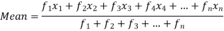
Q9) Find the mean of the following dataset. (5)
x | 20 | 30 | 40 |
f | 5 | 6 | 4 |
A9)
We have the following table-
X | F | Fx |
20 | 5 | 100 |
30 | 6 | 180 |
40 | 7 | 160 |
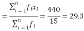
| Sum = 15 | Sum = 440 |
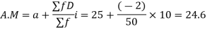
Then Mean will be-
Q10) Find the arithmetic mean for the following distribution (5)
Class | 0-10 | 10-20 | 20-30 | 30-40 | 40-50 |
Frequency | 7 | 8 | 20 | 10 | 5 |
A10)
Let a =25
Class | Mid-value x | Frequency F |  | f.D |
0-10 | 5 | 7 | -2 | -14 |
10-20 | 15 | 8 | -1 | -8 |
20-30 | 25 | 20 | 0 | 0 |
30-40 | 35 | 10 | +1 | +10 |
40-50 | 45 | 5 | +2 | +10 |
Total |
| 50 |
| -2 |
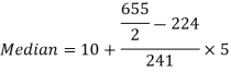
Q11) Find the value of median from the following data- (8)
Number of days for which absent (less than) | 5 | 10 | 15 | 20 | 25 | 30 | 35 | 40 | 45 |
Number of students | 29 | 224 | 465 | 582 | 634 | 644 | 650 | 653 | 655 |
A11)
The given cumulative frequency distribution will first be converted into ordinary frequency as under:
Class interval | Cumulative frequency | Ordinary frequency |
0-5 | 29 | 29=29 |
5-10 | 224 | 224-29=105 |
10-15 | 465 | 465-224=241 |
15-20 | 582 | 582-465=117 |
20-25 | 634 | 634-582=52 |
25-30 | 644 | 644-634=10 |
30-35 | 650 | 650-644=6 |
35-40 | 653 | 653-650=3 |
40-45 | 655 | 655-653=2 |
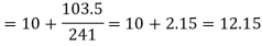
Median = size of 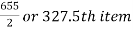
327.5th item lies in 10-15 which is the median class
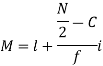
Where l stands for lower limit of median class.
N stands for the total frequency
C stands for cumulative frequency just preceding the median class
i stands for class interval
f stands for frequency for the median class
Q12) A survey was conducted in a housing complex, to find out numbers of person in various age groups, who are using the ATM cards of banks. The result of the survey are as shown below. (5)
Age group | Number of persons |
Below 20 | 10 |
Below 40 | 25 |
Below 60 | 50 |
Below 80 | 70 |
Find the mode of above distribution
A12)
Class interval | Frequencies |
0-20 | 10 |
20-40 | 25-10=15 |
40-60 | 50-25=25 |
60-80 | 70-50=20 |
The maximum frequency 25 is for the class 40-60
Class 40-60 is modal class.
By using formula-
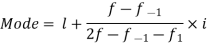
We get-
Mode = 53.3333
Q13) Calculate the first and third quartile of the following data- (5)
Class interval | f |
0-10 | 3 |
10-20 | 5 |
20-30 | 7 |
30-40 | 9 |
40-50 | 4 |
A13)
Class interval | f | CF |
0-10 | 3 | 3 |
10-20 | 5 | 8 |
20-30 | 7 | 15 |
30-40 | 9 | 24 |
40-50 | 4 | 28 |
| N = 28 |
|
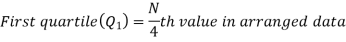
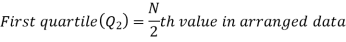
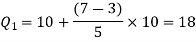
Here N/4 = 28/4 = 7
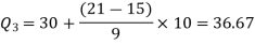
The 7th observation falls in the class 10-20. So, this is the first quartile class. 3N/4 = 21th observation falls in class 30-40, so it is the third quartile class.
For first quartile l = 10, f = 5, C = 3, N = 28
We know that-

For third quartile l = 30, f = 9, C = 15
Q14) What is range? And how do we calculate range and coefficient of range? (5)
A14)
Range is the simplest measure of dispersion. Range is the difference between the maximum value of the variable and the minimum value of the variable in the distribution.

For example:
Find the range of the data- 8, 5, 6, 4, 7, 10, 12, 15, 25, 30
Sol. Here the maximum value is 30 and the minimum value is 4 so that the range is-
30 – 4 = 26
Coefficient of range-
The coefficient of range can be calculated as follows-
Coefficient of Range = 
Q15) What do you understand by QD?(7)
A15)
The quartiles divide a data set into quarters. The first quartile, (Q1) is the middle number between the smallest number and the median of the data. The second quartile, (Q2) is the median of the data set. The third quartile, (Q3) is the middle number between the median and the largest number.
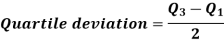
Quartile deviation or semi-inter-quartile deviation is
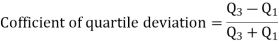
Relative measure of Q.D. Known as Coefficient of Q.D. And is defined as
Q16) Find the quartile deviation of the following data- (8)
Class | 0-5 | 5-10 | 10-15 | 15-20 | 20-25 | 25-30 | 30-35 | 35-40 |
Frequency | 6 | 8 | 12 | 24 | 36 | 32 | 24 | 8 |
A16)
We will construct the cumulative frequency table-
Class interval | f | CF |
0-5 | 6 | 6 |
5-10 | 8 | 14 |
10-15 | 12 | 26 |
15-20 | 24 | 50 |
20-25 | 36 | 86 |
25-30 | 32 | 118 |
30-35 | 24 | 142 |
35-40 | 8 | 150 |
| N = 150 |
|
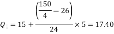
We know that-

So that
And
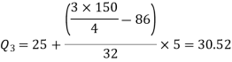
Therefore-
Q = ½ × (Q3 – Q1) = (30.52 – 17.40) / 2 = 6.56
Q17) Find the mean deviation from mean of the following data- (5)
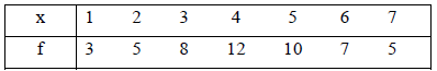
A17)
x | F | Fx | |x-  | f|x-  |
1 | 3 | 3 | 3.24 | 9.72 |
2 | 5 | 10 | 2.24 | 11.20 |
3 | 8 | 24 | 1.24 | 9.92 |
4 | 12 | 48 | 0.24 | 2.88 |
5 | 10 | 50 | 0.76 | 7.60 |
6 | 7 | 42 | 1.76 | 12.32 |
7 | 5 | 35 | 2.76 | 13.80 |
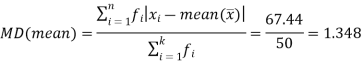
Total | 50 | 212 | 12.24 | 67.44 |
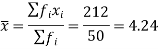
We know that-
Q18) Calculate S.D for the following distribution. (7)
Wages in rupees earned per day | 0-10 | 10-20 | 20-30 | 30-40 | 40-50 | 50-60 |
No. Of Labourers | 5 | 9 | 15 | 12 | 10 | 3 |
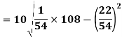
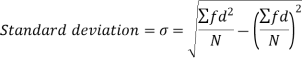
A18)
Wages earned C.I | Mid value  | Frequency |  |  |  |
52 | 5 | 5 | -2 | -10 | 20 |
153 | 15 | 9 | -1 | -9 | 9 |
25 | 25 | 15 | 0 | 0 | 0 |
35 | 35 | 12 | 1 | 12 | 12 |
45 | 45 | 10 | 2 | 20 | 40 |
55 | 55 | 3 | 3 | 9 | 27 |
Total | - |  |  |  |  |
Using formula,