Unit - 3
Classification & Regression
Q1) What is a decision tree?
A1) Decision Tree is a Supervised learning technique that can be used for both classification and Regression problems, but mostly it is preferred for solving Classification problems. It is a tree-structured classifier, where internal nodes represent the features of a dataset, branches represent the decision rules and each leaf node represents the outcome.
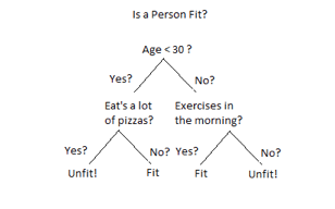
Fig 1: Decision tree example
In a Decision tree can be divided into:
● Decision Node
● Leaf Node
Decision nodes are marked by multiple branches that represent different decision conditions whereas output of those decisions is represented by leaf node and do not contain further branches.
The decision tests are performed on the basis of features of the given dataset.
It is a graphical representation for getting all the possible solutions to a problem/decision based on given conditions.
Decision Tree algorithm:
● Comes under the family of supervised learning algorithms.
● Unlike other supervised learning algorithms, decision tree algorithms can be used for solving regression and classification problems.
● Are used to create a training model that can be used to predict the class or value of the target variable by learning simple decision rules inferred from prior data (training data).
● Can be used for predicting a class label for a record we start from the root of the tree.
● Values of the root attribute are compared with the record’s attribute. On the basis of comparison, a branch corresponding to that value is considered and jumps to the next node.
Issues in Decision tree learning
● It is less appropriate for estimation tasks where the goal is to predict the value of a continuous attribute.
● This learning is prone to errors in classification problems with many classes and relatively small number of training examples.
● This learning can be computationally expensive to train. The process of growing a decision tree is computationally expensive. At each node, each candidate splitting field must be sorted before its best split can be found. In some algorithms, combinations of fields are used and a search must be made for optimal combining weights. Pruning algorithms can also be expensive since many candidate sub-trees must be formed and compared.
- Avoiding overfitting
A decision tree’s growth is specified in terms of the number of layers, or depth, it’s allowed to have. The data available to train the decision tree is split into training and testing data and then trees of various sizes are created with the help of the training data and tested on the test data. Cross-validation can also be used as part of this approach. Pruning the tree, on the other hand, involves testing the original tree against pruned versions of it. Leaf nodes are removed from the tree as long as the pruned tree performs better on the test data than the larger tree.
Two approaches to avoid overfitting in decision trees:
● Allow the tree to grow until it overfits and then prune it.
● Prevent the tree from growing too deep by stopping it before it perfectly classifies the training data.
2. Incorporating continuous valued attributes
3. Alternative measures for selecting attributes
● Prone to overfitting.
● Require some kind of measurement as to how well they are doing.
● Need to be careful with parameter tuning.
● Can create biased learned trees if some classes dominate.
Q2) Write about Random forest?
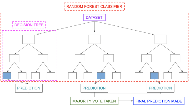
A2) Random forest is an ensemble model in which several trees are grown and objects are classified based on the "votes" of all the trees. In other words, an item is allocated to the class with the greatest votes across all trees. The problem of strong bias (overfitting) could be solved this way. (— courtesy of Kaggle)

Fig 2: Random forest
The random forest classifier is a meta-estimator that fits a number of decision trees on different sub-samples of datasets and utilises average to improve the model's predictive accuracy and control over-fitting. The size of the sub-sample is always the same as the size of the original input sample, but the samples are generated with replacement.
Pros of RF:
● It can handle big data sets with high dimensionality and produce Importance of Variable, which is useful for data exploration.
● Could deal with missing data and retain accuracy.
Cons of RF:
● Users have limited influence over what the model does, therefore it may be a black box.
Classification in random forest
Random forest classification uses an ensemble methodology to achieve the desired result. Various decision trees are trained using the training data. This dataset contains observations and features that will be chosen at random when nodes are split.
Various decision trees are used in a rain forest system. There are three types of nodes in a decision tree: decision nodes, leaf nodes, and the root node. Each tree's leaf node represents the final output produced by that particular decision tree. The final product is chosen using a majority-voting procedure. In this situation, the final output of the rain forest system is the output chosen by the majority of decision trees. A simple random forest classifier is depicted in the diagram below.
Q3) Explain Naive bayes?
A3) The Naïve Bayes algorithm is comprised of two words Naïve and Bayes, Which can be described as:
● Naïve: It is called Naïve because it assumes that the occurrence of a certain feature is independent of the occurrence of other features. Such as if the fruit is identified based on color, shape, and taste, then red, spherical, and sweet fruit is recognized as an apple. Hence each feature individually contributes to identifying that it is an apple without depending on each other.
● Bayes: It is called Bayes because it depends on the principle of Bayes’ Theorem.
Naïve Bayes Classifier Algorithm
Naïve Bayes algorithm is a supervised learning algorithm, which is based on the Bayes theorem and used for solving classification problems. It is mainly used in text classification that includes a high-dimensional training dataset.
Naïve Bayes Classifier is one of the simple and most effective Classification algorithms which help in building fast machine learning models that can make quick predictions.
It is a probabilistic classifier, which means it predicts based on the probability of an Object.
Some popular examples of the Naïve Bayes Algorithm are spam filtration, Sentimental analysis, and classifying articles.
Bayes’ Theorem:
● Bayes’ theorem is also known as Bayes’ Rule or Bayes’ law, which is used to determine the probability of a hypothesis with prior knowledge. It depends on the conditional probability.
● The formula for Bayes’ theorem is given as:

Where,
● P(A|B) is Posterior probability: Probability of hypothesis A on the observed event B.
● P(B|A) is Likelihood probability: Probability of the evidence given that the probability of a hypothesis is true.
● P(A) is Prior Probability: Probability of hypothesis before observing the evidence.
● P(B) is a Marginal Probability: Probability of Evidence.
Working of Naïve Bayes’ Classifier can be understood with the help of the below example:
Suppose we have a dataset of weather conditions and corresponding target variable
“Play”. So using this dataset we need to decide whether we should play or not on a
Particular day according to the weather conditions. So to solve this problem, we need to follow the below steps:
Convert the given dataset into frequency tables.
Generate a Likelihood table by finding the probabilities of given features.
Now, use Bayes theorem to calculate the posterior probability.
Problem: If the weather is sunny, then the Player should play or not?
Solution: To solve this, first consider the below dataset:
Outlook Play
0 Rainy Yes
1 Sunny Yes
2 Overcast Yes
3 Overcast Yes
4 Sunny No
5 Rainy Yes
6 Sunny Yes
7 Overcast Yes
8 Rainy No
9 Sunny No
10 Sunny Yes
11 Rainy No
12 Overcast Yes
13 Overcast Yes
Frequency table for the Weather Conditions:
Weather Yes No
Overcast 5 0
Rainy 2 2
Sunny 3 2
Total 10 5
Likelihood table weather condition:
Weather No Yes
Overcast 0 5 5/14 = 0.35
Rainy 2 2 4/14 = 0.29
Sunny 2 3 5/14 = 0.35
All 4/14=0.29 10/14=0.71
Applying Bayes’ theorem:
P(Yes|Sunny)= P(Sunny|Yes)*P(Yes)/P(Sunny)
P(Sunny|Yes)= 3/10= 0.3
P(Sunny)= 0.35
P(Yes)=0.71
So P(Yes|Sunny) = 0.3*0.71/0.35= 0.60
P(No|Sunny)= P(Sunny|No)*P(No)/P(Sunny)
P(Sunny|NO)= 2/4=0.5
P(No)= 0.29
P(Sunny)= 0.35
So P(No|Sunny)= 0.5*0.29/0.35 = 0.41
So as we can see from the above calculation that P(Yes|Sunny)>P(No|Sunny)
Hence on a Sunny day, the Player can play the game.
Applications of Naïve Bayes Classifier:
● It is used for Credit Scoring.
● It is used in medical data classification.
● It can be used in real-time predictions because Naïve Bayes Classifier is an eager learner.
● It is used in Text classification such as Spam filtering and Sentiment analysis.
Q4) Write the advantages and disadvantages of Naive Bayes?
A4) Advantages of Naïve Bayes Classifier:
● Naïve Bayes is one of the fast and easy ML algorithms to predict a class of datasets.
● It can be used for Binary as well as Multi-class Classifications.
● It performs well in Multi-class predictions as compared to the other Algorithms.
● It is the most popular choice for text classification problems.
Disadvantages of Naïve Bayes Classifier:
● Naive Bayes assumes that all features are independent or unrelated, so it cannot learn the relationship between features.
Q5) What are the types of Naive Bayes models?
A5) Types of Naïve Bayes Model:
There are three types of Naive Bayes Model, which are given below:
Gaussian: The Gaussian model assumes that features follow a normal distribution.
This means if predictors take continuous values instead of discrete, then the model assumes that these values are sampled from the Gaussian distribution.
Multinomial: The Multinomial Naïve Bayes classifier is used when the data is multinomial distributed. It is primarily used for document classification problems, it means a particular document belongs to which category such as Sports, Politics, education, etc.
The classifier uses the frequency of words for the predictors.
Bernoulli: The Bernoulli classifier works similarly to the Multinomial classifier, but the predictor variables are the independent Booleans variables. Such as if a particular word is present or not in a document. This model is also famous for document classification tasks.
Q6) Define a support vector machine?
A6) SVM is another linear classification algorithm (One which separates data with a hyperplane) just like logistic regression and perceptron algorithms.
Given any linearly separable data, we can have multiple hyperplanes that can function as a separation boundary as shown. SVM selects the "optimal" hyperplane of all candidate hyperplanes.
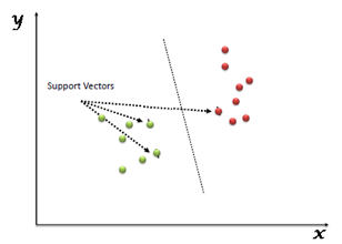
Fig 3: Support vector machine
To understand definition of "optimal" hyperplane, let us first define some concepts we will use
● Margin: It is the distance of the separating hyperplane to its nearest point/points.
● Support Vectors: The point/points closest to the dividing hyperplane.
The optimal hyperplane is defined as the one which maximises the margin. Thus SVM is posed as an optimization problem where we have to maximise margin subject to the constraint that all points lie on the correct side of the separating hyperplane
If all candidate hyperplanes correctly classify the data, why is maximum margin hyperplane the optimal one? One intuitive explanation is - If the incoming samples to be classified contain noise, we do not want them to cross the boundary and be classified incorrectly.
Q7) Write the advantages and disadvantages of a support vector machine?
A7) Advantages:
● It works very well with a clear margin of separation
● It is useful in high dimensional spaces.
● It is useful in situations where the number of dimensions is greater than the number of samples.
● It uses a subset of training points in the decision function (called support vectors), so it is also memory efficient.
Disadvantages:
● It doesn’t work well when we have a broad data set because the necessary training time is higher.
● It also doesn’t work very well, when the data set has more noise i.e. target classes are overlapping.
● SVM doesn’t explicitly have probability estimates, these are determined using a costly five-fold cross-validation.
Q8) Explain logistic regression?
A8) Another approach to linear classification is the logistic regression model, which, despite its name, is a classification rather than a regression system.
In Logistic regression, we take a weighted linear combination of input features and pass it through a sigmoid function which outputs a number between 1 and 0. Unlike perceptron, which only tells us which side of the plane the point lies on, logistic regression gives a likelihood of a point lying on a particular side of the plane.
The probability of classification would be very similar to 1 or 0 as the point goes far away from the plane. The chance of classification of points very close to the plane is close to 0.5.

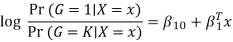
Fig 4: Logistic regression
The model is defined in terms of K-1 log-odds ratios, with an arbitrary class chosen as reference class (in this example it is the last class, K) (in this example it is the last class, K). Consequently, the difference between log-probabilities of belonging to a given class and to the reference class is modelled linearly as

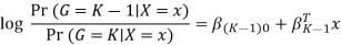
Where G stands for the real, observed class. From here, the probabilities of an observation belonging to each of the groups can be determined as
That clearly shows that all class probabilities add up to one.
Logistic regression models are usually calculated by maximum likelihood. Much as linear models for regression can be regularised to increase accuracy, so can logistic regression. In reality, L2 penalty is the default setting. It also supports L1 and Elastic Net penalties (to read more on these, check out the link above), but not all of them are supported by all solvers.
Q9) Explain k - means?
A9) K-Means Clustering is an unsupervised learning approach used in machine learning and data science to solve clustering problems. K specifies the number of predefined clusters that must be produced during the process; for example, if K=2, two clusters will be created, and if K=3, three clusters will be created, and so on.
It allows us to cluster data into different groups and provides a simple technique to determine the categories of groups in an unlabeled dataset without any training.
It's a centroid-based approach, which means that each cluster has its own centroid. The main goal of this technique is to reduce the sum of distances between data points and the clusters that they belong to.
For numeric results, K-Means clustering is one of the most commonly used prototype-based clustering algorithms. The centroid or mean of all the data points in a cluster is the prototype of a cluster in k-means. As a consequence, the algorithm works best with continuous numeric data. When dealing with data that includes categorical variables or a mixture of quantitative and categorical variables.
The technique takes an unlabeled dataset as input, separates it into a k-number of clusters, and continues the procedure until no better clusters are found. In this algorithm, the value of k should be predetermined.
The k-means clustering algorithm primarily accomplishes two goals:
● Iteratively determines the optimal value for K centre points or centroids.
● Each data point is assigned to the k-center that is closest to it. A cluster is formed by data points that are close to a specific k-center.
As a result, each cluster contains datapoints with certain commonality and is isolated from the others.
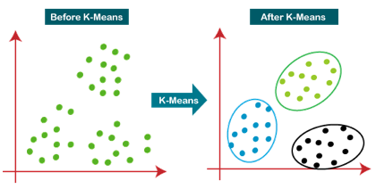
Fig 5: Working of the K-means Clustering Algorithm
Pseudo Algorithm
- Choose an appropriate value of K (number of clusters we want)
- Generate K random points as initial cluster centroids
- Until convergence (Algorithm converges when centroids remain the same between iterations):
● Assign each point to a cluster whose centroid is nearest to it ("Nearness" is measured as the Euclidean distance between two points)
● Calculate new values of centroids of each cluster as the mean of all points assigned to that cluster
Advantages
Some of the benefits of K-Means clustering techniques are as follows:
● It is simple to comprehend and implement.
● K-means would be faster than Hierarchical clustering if we had a high number of variables.
● An instance can modify the cluster when centroids are recalculated.
● When compared to Hierarchical clustering, K-means produces tighter groupings.
Disadvantages
Some of the drawbacks of K-Means clustering techniques are as follows:
● The number of clusters, or the value of k, is difficult to anticipate.
● Initial inputs such as the number of clusters have a significant impact on output (value of k).
● The order in which the data is entered will have a significant impact on the final result.
● It is very sensitive to rescaling. If we will rescale our data by means of normalization or standardization, then the output will completely change.
● It is not good in doing clustering job if the clusters have a complicated geometric shape.
Q10) Describe KNN?
A10) It is one of the simplest Machine Learning algorithms based on Supervised Learning technique.
- Algorithm assumes the similarity between the new case/data and available cases, puts the new case into the category that is most similar to the available categories.
- Algorithm stores all the available data and classifies a new data point based on the similarity. This means when new data appears then it can be easily classified into a well suite category by using K NN algorithm.
- Algorithm can be used for Regression and Classification but mostly it is used for the Classification type problems.
- It is a non-parametric algorithm, which means it does not make any assumption on underlying data.
- It is known as lazy learner algorithm because it does not learn from the training set immediately instead it stores the dataset and at the time of classification, it performs an action on the dataset.
- Algorithm at the training phase just stores the dataset and when it gets new data, then it classifies that data into a category that is much similar to the new data.
Importance of KNN Algorithm
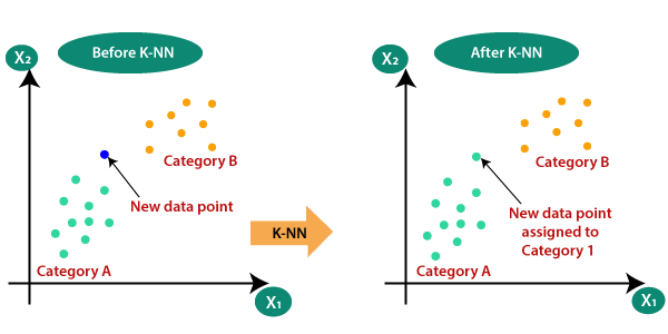
Consider there are 2 categories, that is Category A and Category B, and we have a new data point x1, so this data point will lie in which of these categories. To solve this type of problem, we need algorithm. With the help of algorithm, we can easily identify the category or class of a particular dataset. Consider the below diagram.
The K-NN working can be explained on the basis of the below algorithm.
Step-1: Select the number K of the neighbors
Step-2: Calculate the Euclidean distance of K number of neighbors
Step-3: Take the K nearest neighbors as per the calculated Euclidean distance.
Step-4: Among these k neighbors, count the number of the data points in each category.
Step-5: Assign the new data points to that category for which the number of the neighbor is maximum.
Step-6: Our model is ready.
Q11) Write the difference between classification and regression?
A11) Difference between Classification and Regression
Regression Algorithm | Classification Algorithm |
In Regression, the output variable must be of continuous nature or real value. | In Classification, the output variable must be a discrete value. |
The task of the regression algorithm is to map the input value (x) with the continuous output variable(y). | The task of the classification algorithm is to map the input value(x) with the discrete output variable(y). |
Regression Algorithms are used with continuous data. | Classification Algorithms are used with discrete data. |
In Regression, we try to find the best fit line, which can predict the output more accurately. | In Classification, we try to find the decision boundary, which can divide the dataset into different classes. |
Regression algorithms can be used to solve the regression problems such as Weather Prediction, House price prediction, etc. | Classification Algorithms can be used to solve classification problems such as Identification of spam emails, Speech Recognition, Identification of cancer cells, etc. |
The regression Algorithm can be further divided into Linear and Non-linear Regression. | The Classification algorithms can be divided into Binary Classifier and Multi-class Classifier. |
Q12) Write the difference between K-means and KNN?
A12) Difference between K-means and KNN
● KNN is a Supervised machine learning while K-means is an unsupervised machine learning.
● KNN is a machine learning algorithm for classification or regression, whereas K-means is a clustering machine learning technique.
● KNN is a slacker when it comes to learning, whereas K-Means is a fast learner. An enthusiastic learner has a model fitting, which indicates a training phase, whereas a lazy learner does not.
● KNN performs much better if all of the data have the same scale but this is not true for K-means.


