UNIT 5
Ans
ADVANTAGES OF SQC
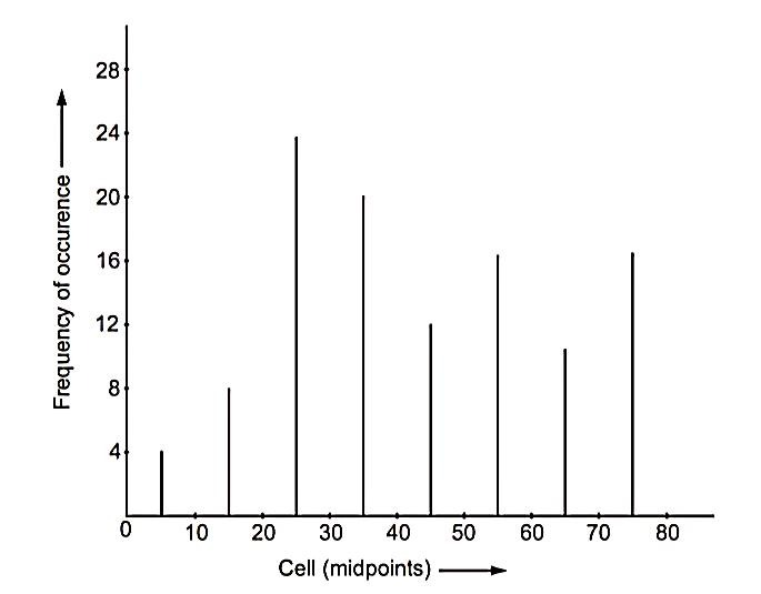
2. Draw & explain different frequency diagrams.
Ans

2. Frequency Polygon

3. Bar Chart
3. Explain the procedure of plotting X̅ and R Chart
Ans
Step – I: Calculate Average ( X̅) and Range (R) for each sample.

x̿ = 
& 
where N = Number of samples
The control limits are given by,
Upper control limit X̅ = UCL X̅ = x̿ + 3σ X̅
Lower control limit X̅ = LCL X̅ = x̿ - 3σ X̅
Here, σ. X̅ = Standard deviation of averages = 
Where n = sample size
σ' = Standard deviation of universe = 
where, d2 is a factor depending upon sample size.
(i) UCL R = D4  and LCL R = D3
(ii) UCL R = D2 σ’ and LCL R = D1 σ’
(i) For X̅ chart, the central line on X̅ chart should be drawn as solid horizontal line as x̿. The upper and lower control limits should be drawn as dotted horizontal lines at the calculated values.
(ii) For R chart, central line on R chart should be drawn as solid horizontal line as  and control limits should be drawn as dotted horizontal lines.
The values of X̅1, X̅2, X̅3… X̅4 are plotted on X̅ chart, whereas, values of R1, R2, R3, … Rn are plotted on R chart. Points falling outside the control limits are indicated by cross, whereas, points falling inside the control limits are encircled.
4. State objectives & limitations of X̅ and R-chart.
Ans: Objectives of X̅ and R-chart
Limitations of X̅ and R-chart
5. Explain the procedure of plotting P-Chart & state objectives of P chart.
Ans: Steps to Draw P-Chart
P = 
3. Compute  (Average fraction defective) as,
 =
= 
4. Compute control limits,
UCL P = 
LCL P = 
5. Plot each point as obtained and control limits as calculated. The points falling outside control limits are identified, (If any).
6. If the points fall outside the control limits, there may be two reasons:
(a) Assignable causes of variation may be present.
(b) Standard of Quality level is different for assumed standard P.
Objectives of P-Chart
Because of lower inspection and maintenance costs of P-chart, they usually have a greater area of economical applications than control charts used for variable.
6. Explain the procedure of plotting C-Chart & state applications of C chart.
Ans
We have, Central line =  =
= 
Upper control limit, UCL C = 
Lower control limit, UCL C = 
Applications of C Chart
(a) Number of surface defects in an aircraft wing.
(b) Number of defects such as blowholes, cracks in a casting.
(c) Number of imperfections observed in a cloth of unit area.
(d) Number of surface defects in galvanized sheet.
(e) Number of small holes in glass bottles.
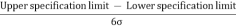
7. Explain different Process capability Indices.
Ans: Cp :-
• Process capability ratio or index is given by,
Cp = 
= 

Cpk :-
Cpk = min
Ppk :-
Ppk = min 
8. Explain PPAP & state its advantages.
Ans
Advantages of PPAP
Improves the overall quality of product.
9. Explain sampling inspection & state its advantages & limitations.
Ans
1. 100% inspection.
2. Sampling inspection or Acceptance sampling.
Advantages of Acceptance Sampling:
(i) The method is applicable in those industries where there is mass production and the industries follow a set production procedure.
(ii) The method is economical and easy to understand.
(iii) Causes less fatigue boredom.
(iv) Computation work involved is comparatively very small.
(v) The people involved in inspection can be easily imparted training.
(vi) Products of destructive nature during inspection can be easily inspected by sampling.
(vii) Due to quick inspection process, scheduling and delivery times are improved.
Limitations of Acceptance Sampling:
(i) It does not give 100% assurance for the confirmation of specifications so there is always some likelihood/risk of drawing wrong inference about the quality of the batch/lot.
(ii) Success of the system is dependent on, sampling randomness, quality characteristics to be tested, batch size and criteria of acceptance of lot.
10. Explain O.C. curve & state its characteristics & Significance.
Ans

2. Indifference quality region
3. Objectionable quality region.
Characteristics of O.C. Curve
Significance of O.C. Curve
11. Explain different sampling methods
Ans
b. Stratified Sampling
c. Cluster Sampling
d. Sampling in Stages
12. Explain different sampling plans.
Ans
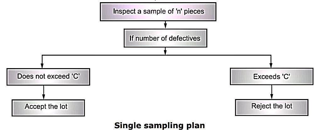
1. N = Lot size,
2. n = Sample size,
3. C = Acceptance number = Maximum number of allowable defectives in sample of size 'n'.
2. Double Sampling Plan
Let n1 = Number of pieces in the first sample
C1 = Acceptance number for the first sample = Maximum number of defectives, that will permit the acceptance of lot on the basis of first sample.
n2 = Number of pieces in the second sample.
n1 + n2 = Number of pieces in the two samples combined.
C2 = Acceptance number for the two samples combined = Maximum number of defectives, that will permit the acceptance of lot on the basis of first and second sample combined.
Advantages/Merits of Double Sampling Plan:
1. It gives second chance to the producer. Therefore, it is much preferred and acceptable to producers.
2. Cost of administration is moderate.
Disadvantages/Demerits:
1. Economical loss, if
(i) Samples do not represent the true picture of lot, and
(ii) Acceptance criteria (number) is not selected properly.
2. More record keeping is required, since decision is made on two samples drawn and number of parameters stated are more.

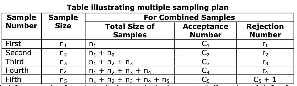
3. Multiple Sampling Plans
(i) A first sample of n1 pieces is drawn, the lot is accepted, if number of defectives are less than C1 and rejected, if more than r1.
(ii) But, if C1 < defectives < r1, a second sample of n2 pieces is drawn, the lot is accepted, if number of defectives are less than C2 in combined sample of ‘n1 + n2’ and rejected, if more than r2. The procedure is continued in accordance with the above table.
(iii) If by the end of fourth sample, the lot is neither accepted nor rejected, a sample of n5 pieces is drawn.
(iv) The lot is accepted, if the number of defectives in the combined sample of n1, n2, n3, n4, n5 is less than C5 and rejected, if more than C5 + 1.
13. Compare different sampling plan.
Ans
Sr. No. | Feature | Single | Double | Multiple |
1 | Average number of | Generally large. | In between single and multiple. It is preferred to take second sample of size twice the size of first sample. | Low. |
2 | Acceptability to producer. | Poor, as it gives only one chance to decide, whether the lot is accepted or rejected | Most acceptable (Gives II nd chance). | Less acceptable, if indecision continues for a long period and more number of samples are drawn for making decision. |
3 | Cost of Administration | Lowest. | In between. | Largest. |
4 | Information available about prevailing quality level. | Largest. | In between. | Lowest. |
5 | Number of samples | One | Two | Multiple. |
6 | Variability of inspection load [i.e. number of items undergoing inspection] | Constant | Variable, depending upon behaviour of first sample. | Highly variable. |
7 | Estimation about quality of a lot | Best | Intermediate | Difficult to estimate. |
8 | Decision of 'Acceptance' or 'Rejection' is based on | One sample | Two samples combined. | Multiple samples combined. |
14. Explain AOQ.
Ans.
AOQ = Pa · p’ 
where, Pa = Probability of acceptance
N = Lot size
n = Sample size


