Unit - 1
Discrete-time signals and systems
Q1) For sequence h[n]={ 1, 2 , 1, -1} determine the response of system with input signal x[n] = {1, 2 ,3 ,1}
a) Finding x[k] and h[k] i.e n=k.
b) Folding h[k] we get h[-k].
c) Then shifting the above signal[-k] we get h[1-k]
d) Multiplying above signal h[1-k] with x[n].
e) Again, incrementing h[1-k] by 1 we get h[2-k] multiplying with x[n].
f) Continuing this process till we get 0 for output y. In this case for n=5.
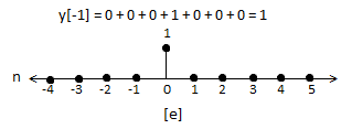
A1) The graphical representation is shown below.


Q2) For h[n] = {1, 2, 1, -1}, x[n] = {1, 2, 3, 1}. Find x[n]*h[n]?
A2)
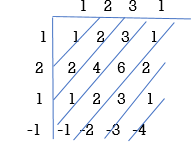
y[-1] = 1
y[0]= 2+2 = 4
y[1] = 1+4+3 = 8
y[2]= -1+2+6+1 = 8
y[3]= -2+3+2 = 3
y[4]= -3+1 = -2
y[5]= -1
y[n]= {1, 4, 8, 8, -2, -1}
The above sequence is the required convolution of x[n] and h[n].
Q3) Determine if the system y(n) = T[x(n)] = x(–n) is linear or nonlinear.
A3) Determine the outputs y1(n) and y2(n) corresponding to the two input sequences x1(n) and x2(n) and form the weighted sum of outputs:
y1(n) = T[x1(n)] = x1(–n) y2(n) = T[x2(n)] = x2(–n)
The weighted sum of outputs = a1 x1(–n) + a2 x2(–n) ‹(A).
Next determine the output y3 due to a weighted sum of inputs:
y3(n) = T[a1 x1(n) + a2 x2(n)] = a1 x1(–n) + a2 x2(–n) <(B)
Check if (A) and (B) are equal. In this case (A) and (B) are equal; hence the system is linear.
Q4) Examine y(n) = T[x(n)] = x(n) + n x(n+1) for linearity.
A4) The outputs due to x1(n) and x2(n) are:
y1(n) = T[x1(n)] = x1(n) + n x1(n+1)
y2(n) = T[x2(n)] = x2(n) + n x2(n+1)
The weighted sum of outputs = a1 x1(n) + a1 n x1(n+1) + a2 x2(n) + a2 n x2(n+1) <(A)
The output due to a weighted sum of inputs is
y3(n) = T[a1 x1(n) + a2 x2(n)]
= a1 x1(n) + a2 x2(n) + n (a1 x1(n+1) + a2 x2(n+1))
= a1 x1(n) + a2 x2(n) + n a1 x1(n+1) + n a2 x2(n+1) <(B)
Since (A) and (B) are equal the system is linear.
Q5) Check the system y(n) = T[x(n)] = ne |x(n)| for linearity.
A5) The outputs due x1(n) and x2(n) are:
y1(n) = T[x1(n)]= n e |x1 (n)|
y2(n) = T[x2(n)] = n e|x2 (n)|
The weighted sum of the outputs = a1 ne|x1 (n)|+ a n e|x2 (n)| <(A)
The output due to a weighted sum of inputs is y3(n) =T[a1 x1(n) + a2 x2(n)] = n e|a1 x1 (n)|+|a2x1 (n)| <(B) We can specify a1, a2, x1(n), x2(n) such that (A) and (B) are not equal. Hence nonlinear.
Q6) Check the system y(n) = T[x(n)] = n x(n) for linearity.
A6) For the two arbitrary inputs x1(n) and x2(n) the outputs are
y1(n) = T[x1(n)] = n x1(n)
y2(n) = T[x2(n)] = n x2(n)
For the weighted sum of inputs a1 x1(n) + a2 x2(n) the output is
y3(n) = T [a1 x1(n) + a2 x2(n)] = n (a1 x1(n) + a2 x2(n)) = a1 n x1(n) + a2 n x2(n) = a1 y1(n) + a2 y2(n). Hence the system is linear.
Q7)For x(t) indicated in figure 1 sketch the following
(a) x(-t)
(b) x(t+2)
(c) x(2t+2)
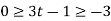
(d) x(1-3t)
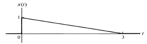
A7)
(a) This is just a time reversal

Note: Amplitude remains the same. Also reversal occurs about t=0
(b) This is a shift in time. At t=-2, the vertical portion occurs.

(c)A scaling by a factor of 2 occurs as well as time shift


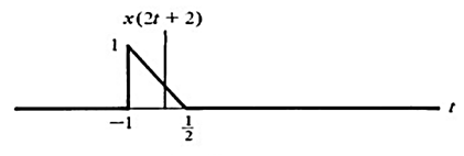
Note: a>1 induces a compression
(d) All three effects are combined in this linear scaling.


Q8) For y(t)=cos[x(t)], comment whether it is time invariant or not?
A8) From model 1


Y(t)=cos[x(t-t0)]
From model 2


Y(t)=cos[x(t-t0)]
Since, time delay or advance in the input signal produces the corresponding change in the output. Hence, it is time invariant.
Q9) For y(t)=x(t2), is the system causal or anti causal?
A9) y(t)= x(t2)
If the output for any time depends on the future than its not causal. So, Let t=1
Y(1)=x(1)
t=2
y(2)=x(4)
Since, it depends on future values, so it is anti-causal.
Q10) For y(t)=x(t)+2. Comment whether system has memory or memoryless?
A10) For t=1
Y(1)=x(1)+2
For t=2
Y(2)=x(2)+2
So, for any value of t the output depends only on present input. Hence, it is memoryless.
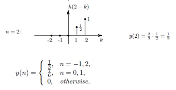
Q11) Let us find the response to  . The impulse response h of the system is the response to the unit impulse:

A11)
(1) flip h;
(2) for a fixed n, shift h by n;
(3) for the same fixed n, multiply x(k) by h(n-k), for each k;
(4) Sum the products over k; 

Q12) Compare analog and digital signals?
A12)
S.No | Analog signal | Digital signal |
1 | Analog signals are continuous signals. | Digital signals are discrete signals. |
2 | Analog signal uses continuous values for representing the information. | A digital signal uses discrete values for representing the formation. |
3. | Analog signal uses continuous vlaues for representing the information. | A digital signal cannot be affected by the noise during transmission. |
4 | Accuracy of Analog signal is affected by the noise. | Digital signals are noise-immune hence there accuracy is less affected. |
5 | Devices which are using analog signals are less flexible | Device using digital signals are very flexible. |
6 | Analog signals consumes less bndwidth | Digital signals consume more bandwidth |
7 | Analog signal are stored in the form of continuous wave form. | Digital signals are stored in the form of binary bits “0”, “1”. |
9 | Analog signals have low cost. | Digital signals have high cost. |
10 | Analog signals give observation error. | Digital signals doen’t give observaiton error. |
Q13) Compare Digital signals and discrete signals?
A13)
S. No | Discrete-time signal | Digital signal |
1. | The discrete-time signal is a digital representation of a continuous time signal. | The digital signal is form of discrete-time signal. |
2. | The discrete-time signal can be obtained from the continuous-time signal by the Euler’s method. | The digital signal can be obtained by the process of sampling, quantizations, and encoding of the discrete-time signal. |
3. | The discrete-time signal sia signal that has discrete in time and discrete in amplitude. | The digital signal is a signal that has discrete in amplitude and continuous in time. |
4 | The value of the signal can be obtained only at sampling instants of time. | The amplitude signal of the digital signal is either 1 or 0. That is either OFF or ON. |
5 | The signals are sampled but not necessary to quantized in the discrete-time signals. | The signals are sampled and quantized in the digital signals. |
6. | All the discrete-time signals are digital signals. | All the digital signals are not discrete-time signals. |
Q14) For the system with y(t)=x(-t), find whether the system is linear or not?
A14) To comment on linearity of system it should follow law of superposition. So, From model given below
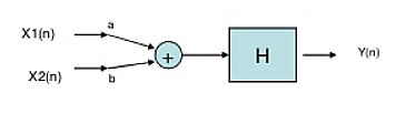
Y(t)=ax1(-t)+bx2(-t)
Now from second model

Y(t)= ax1(-t)+bx2(-t)
Since, output from both the model is same so system is linear.
Q15) What is linear time invariant system? Derive the expression for impulse response of LTI systems?
A15) A LTI system is one which possesses property of linear as well as time invariant system. Linear systems are one which obeys superposition theorem. There are few advantages of using LTI systems, some of which are
i) The LTI system can be easily solved mathematically for both continuous and discrete time systems.
Ii) Accurate modelling is possible in LTI system.
Iii) They are helpful for system design.
Analysis of LTI system is mainly done in two ways
a) Convolution Sum.
b) Difference Equation.
Impulse response
The LTI system can be represented by its impulse response with x(t) as its input signal and y(t) as its output.

Fig: LTI System
Let input signal be x[n]
x[n] = 
The output obtained when we apply input as unit sample sequence for n=k
y[n,k] = h[n,k] = H[ [n-k]]
y[n] = H[x[n]]
= H [  ]
]
But y[n,k] = h[n,k] = H[ [n-k]]
Hence, the output will now be
y[n] = [  ]
]
=  ]
]
Q16) Derive the output equation for convolution sum of LTI systems?
A16) Considering an LTI system with input as impulse signal. As we know that impulse response of any system gives complete describes the behavior of any LTI system. Basically, we decompose the input signal first. The apply input as impulse and obtain the corresponding output. Obtained output is then graphically analysed.
Let input signal be x[n]
x[n] = 
The output obtained when we apply input as unit sample sequence for n=k
y[n,k] = h[n,k] = H[ [n-k]]
Where n= time index
k = location of input impulse parameter
The x[n] because of input weighted sum of output will be
y[n] = H[x[n]]
= H [  ]
]
But y[n,k] = h[n,k] = H[ [n-k]]
Hence, the output will now be
y[n] = [  ]
]
=  ] (Due to superposition theorem)
Now, by time invariance property we can write
h[n]= H [
For delayed sequence we have
h[n-k] =H [ ]
]
Hence, the output equation can now be written as
y[n] = [  ]
]
The above equation is called as convolution sum.
y[n]= x[n] * h[n]
Q17) List the properties of linear convolution?
A17) Commutative Law
x(n) * h(n) = h(n) * x(n)


Associate Law
[ x(n) * h1(n) ] * h2(n) = x(n) * [ h1(n) * h2(n) ]


Distribute Law
x(n) * [ h1(n) + h2(n) ] = x(n) * h1(n) + x(n) * h2(n)
Q18) What is periodic sampling of signals explain with proper waveforms?
A18) Sampling usually refers to conversion of continuous signal into short duration of pulses each pulse followed by a skip period when no signal is available. Below shown is a uniformly sampled signal.
Following are two popular sampling operations:
1. Single rate or periodic sampling
2. Multi-rate sampling
Figure below shows the structure and operation of a finite pulse width sampler, where (a) represents the basic block diagram and (b) illustrates the function of the same. T is the sampling period and p is the sample duration.
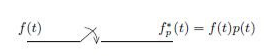

Figure (a): Basic block diagram
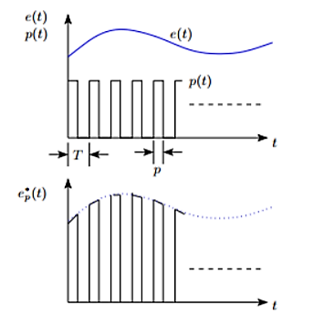
Figure (b): Sampler output
Finite pulse width sampler converts a continuous time signal into a pulse modulated or discrete signal. The most common type of modulation in the sampling and hold operation is the pulse amplitude modulation.
The block diagram of sampler is shown above, having a pulse train of p seconds and sampling period of T seconds.
p(t)= unit pulse train with period T
p(t)=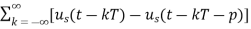
Us(t)=unit step function

In frequency domain p(t) can be represented as
p(t)= 
 = 2π/T
Cn=
p(t)=1 for 0≤ t ≤p
The output of the ideal sampler can be expressed as
f*(t)=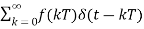
F*(s)=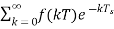
The output of the sampler can be approximated as
Cn=
=
Q19) How are band limited signals recovered explain with proper equations and waveforms?
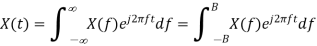
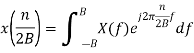
A19) x(t) is Band-limited, with its Fourier transform X(f) being non-zero only in [-B, B]. The dual reasoning of the discussion in previous slide will imply that we can reconstruct X(f) perfectly in [-B, B] by using only the samples x(n / 2B).
Now
 is the -nth Fourier Series Coefficient
  the periodic extension of X(f).


The Fourier inverse of e-j2πto is  (t-to). Therefore, the Fourier inverse
 is
is


Thus, we see that if we multiply the original Band-limited signal with a periodic train of impulses (period 1/2B, with impulse at the origin of strength 1/2B) we obtain a signal whose Fourier transform is a periodic extension of the original spectrum. We need a mechanism that will blank out the spectrum of  in |f|> B, i.e: multiply the spectrum with:

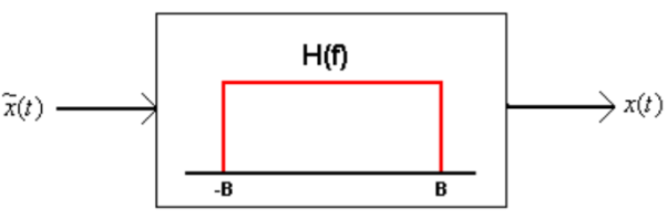
In other words, we need to feed  to an LSI system, the Fourier transform of whose impulse response is the above function (recall the convolution theorem), i.e: one whose impulse response is

Q20) What is quantisation? Explain in detail quantisation in digital sampling?
A20) Quantizing/encoding is the process of mapping the sampled analog voltage values to discrete voltage levels, which are then represented by binary numbers (bits). This is needed because the analog sample values are real numbers that occur on a continuum. That is, for example, if a sine wave of amplitude 1V is being sampled, the sample values could be any value between -1V and +1V… an infinite number of possibilities. In any digital system, there is only a finite amount of memory, so only a finite number of values can be used to represent the samples of the analog signal. Converting a sample value from the set of infinite possibilities to one of a finite set of values is called quantization or quantizing. These values are referred to as quantization levels.
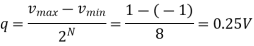
Inputs to A/D converters are limited to a specific voltage range. For the sine wave example above, we assumed that all values of the analog input fall within a range of -1.0 to +1.0 volts (note: this is the typical voltage range of voice or music signals on a computer, such as in .wav or .mp3 files). A/D systems are characterized by the number of bits they have available to perform quantization. The number of bits determines the number of quantization levels. An N-bit A/D converter has 2N quantization levels and outputs binary words of length N (that is, it outputs N-bit values for every sample). For example, a 3-bit A/D system has 23 = 8 quantization levels, so all samples of a 1V analog signal that is input to this A/D will be quantized into one of only 8 possible quantization levels and each sample will be represented by a 3-bit digital word. In general, the A/D converter will partition a range of voltage from some vmin to some vmax into 2N voltage intervals, each of size q volts, where

Some common examples of A/D quantizing are digital telephony, which uses 8-bit A/D (28 = 256 quantization levels), CD audio, which uses 16-bit A/D (216 = 65,536 quantization levels), and DVD audio, which uses 24-bit A/D (224 = 16,777,216 quantization levels). The following figures represent conceptually how a 3-bit A/D converter converts an analog signal into bits. In these figures, the analog signal is shown as well as the samples, with samples taken every 0.5 msec (corresponding to a sample rate of fs = 1/0.0005 sec = 2000 samples/sec). The actual analog sample voltages are shown in parentheses next to the samples. Here, the voltage range of the signal is divided into 23 = 8 smaller voltage intervals (also called steps). These are separated by the dashed, bold horizontal lines, and each interval is 0.25V wide:
The value of q is more formally called the quantizer’s resolution.
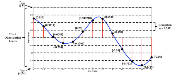
Each of the voltage intervals is assigned an N-bit binary number representing the integers from 0 to 2N-1. For this example, you can see that since we are using a 3-bit A/D, the intervals will be assigned binary numbers representing the integers from 0 to 7 (that is, 000, 001, 010, …, 111), starting from the bottom of the voltage range. In this case, the digital word 000 is assigned to the voltages from -0.75 V to -1.0 V, 001 is assigned to the voltages from -0.5 V to -0.74999 V, and so on. The figure that follows shows for each quantization interval the associated 3-bit digital word (on the left side of the plot). Any analog sample that falls in a given voltage interval will result in those 3 bits being transmitted.

Encoding
When a sample point falls within a given interval, it is assigned the corresponding binary word (this is the Encoding part of Quantization/Encoding). For the first sample point at time 0, the voltage is 0.613 V, which means that sample is assigned a binary value of 110. The A/D then creates a voltage signal that represents these bits, and that process continues as long as an analog signal is input to it. The binary representation of the above signal is:
110 101 100 011 011 100 110 110 100 010 000 000 001.
In this example, every sample produces 3 bits (that is, there are 3 bits/sample). The sample rate was 2000 samples/sec. Multiplying these two values together results in the bit rate (Rb) produced from this A/D conversion:

Bitrate is the speed of transfer of data given in number of bits per second. To the right of the plot above is the quantization level associated with each voltage interval. Any analog sample voltage that falls in a given interval is effectively estimated to the center of its quantization level when it is desired to reconstruct the analog signal from the received bits (a receiver may perform this). This process is referred to as Digital-to-Analog conversion (D/A) and will be discussed briefly in the next section. For this example, the quantization level for the lowest voltage interval is the value halfway between -.75 V and -1 V (which is -0.875 V). This means that any analog sample that fell into this range will be represented as -0.875 V.


