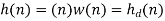
Unit - 4
Structure and Implementation of FIR and IIR Filter
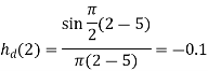
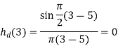
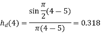
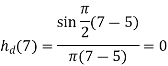
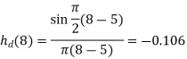
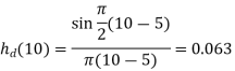
Q1) Design a LPF using rectangular window for the desired frequency response of a low pass filter given by ωc = π/2 rad/sec, and take M=11. Find the values of h(n). Also plot the magnitude response.
A1)

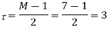
r= M-1/2 = 5
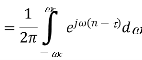
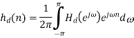
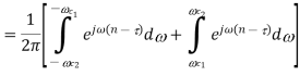
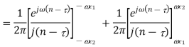
By taking inverse Fourier transform


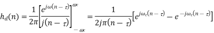

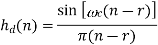
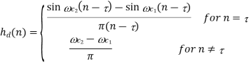
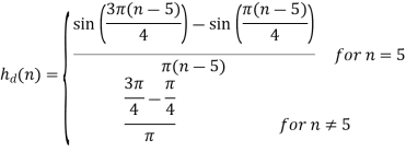
For  and
and 

For 
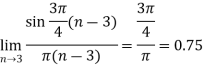
 Using L’Hospital Rule


Where 


The given window is rectangular window ω(n) = 1 for 0 ≤ n ≤ 10
=0 Otherwise
This is rectangular window of length M=11. h(n) = hd (n)ω(n) = hd (n) for 0 ≤ n ≤ 10
H[z]=  =
= 
The impulse response is symmetric with M=odd=11


 |  |  |
           |            |            |
Response

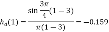
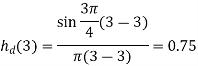
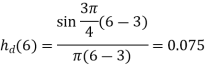
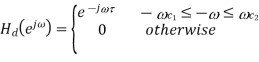
Q2) The desired frequency response of low pass filter is given by Hd (ejω) = e−j3ω − 3π/ 4 ≤ ω ≤ 3π/ 4 and 0 for 3π /4 ≤ |ω| ≤ π Determine the frequency response of the FIR if Hamming window is used with N=7
A2)


For  and
and 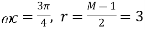

For 
 Using L’Hospital Rule
Where 


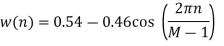
The given window is hamming window


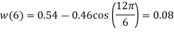
To calculate the value of h(n)


The frequency response is symmetric with M=odd=7


 |  |  |
           |            |        |
RESPONSE

Q3) Design the FIR filter using Hanning window
A3)


To calculate the value of 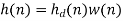


Q4) Design an FIR filter (lowpass) using rectangular window with passband gain of 0 dB, cut-off frequency of 200 Hz, sampling frequency of 1 kHz. Assume the length of the impulse response as 7.
A4)

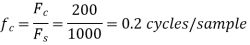


When 

When 

Calculating h(n)
As it is rectangular window h(n) = w(n)=hd(n)=h(n)
For M=7
n |  |
0 | -0.062341 |
1 | 0.093511 |
2 | 0.302609 |
3 | 0.4 |
4 | -0.062341 |
5 | 0.093511 |
6 | 0.302609 |
Q5) Using rectangular window design a lowpass filter with passband gain of unity, cut-off frequency of 1000 Hz, sampling frequency of 5 kHz. The length of the impulse response should be 7.
A5)

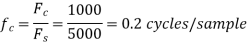


The filter specifications (ωc and M=7) are similar to the previous example. Hence same filter coefficients are obtained.
h (0) =-0.062341, h(1)=0.093511, h(2)=0.302609 h(3)=0.4, h(4)=0.302609, h(5)=0.093511, h(6)=-0.062341
Q6) Design a HPF using Hamming window. Given that cut-off frequency the filter coefficients hd (n) for the desired frequency response of a low pass filter given by ωc = 1rad/sec, and take M=7. Also plot the magnitude response.
A6)

By taking inverse Fourier transform


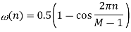
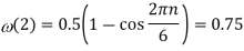
The given window function is Hamming window. In this case
 for
for 

 |  |
0 | -0.00119 |
1 | -0.00448 |
2 | -0.2062 |
3 | 0.6816 |
4 | -0.00119 |
5 | -0.00448 |
6 | -0.2062 |
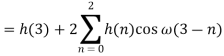
The magnitude response of a symmetric FIR filter with  is
is

For M=7


Q7) Design an ideal bandpass filter having frequency response Hde (jω) for π/ 4 ≤ |ω| ≤ 3π/ 4. Use rectangular window with N=11 in your design.
A7)


The length of the filter with given is related by

And 
The given window is rectangular hence
For n=0,1,2,…,10 estimate the FIR filter coefficients h(n).
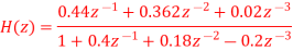
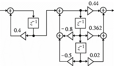
Q8) For the following LTI system H(z)= . Realise the cascade form IIR filter.
A8) H(z)=
The above function can be simplified as
H(z)=
Hence, using the above structure and placing the values of 
 …. And similarly,
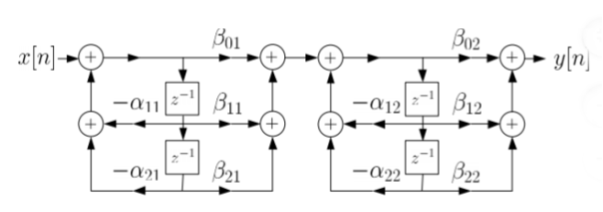
Fig: Cascade Form realisation of IIR Filter
Q9) Draw block diagram for the function using parallel form H(z)=
A9) H(z)=
Writing above transfer function in standard form for parallel realisation we get
H(z)=-20+
The structure is shown below

Q10) Compare IIR and FIR filters?
A10)
S.No | IIR system | FIR system |
1. | IIR stands for infinite impulse response systems | FIR stands for finite impulse response systems |
2. | IIR filters are less powerful that FIR filters, & require less processing power and less work to set up the filters | FIR filters are more powerful than IIR filters, but also require more processing power and more work to set up the filters |
3. | They are easier to change “on the fly”. | They are also less easy to change “on the fly” as you can by tweaking (say) the frequency setting of a parametric (IIR) filter |
4. | These are less flexible. | Their greater power means more flexibility and ability to finely adjust the response of your active loudspeaker. |
5. | It cannot implement linear-phase filtering. | It can implement linear-phase filtering. |
6. | It cannot be used to correct frequency-response errors in a loudspeaker | It can be used to correct frequency- response errors in a loudspeaker to a finer degree of precision than using IIRs. |
Q11) Realise Direct form II and cascade form realizations of
A11) 


Direct form II
Cascade form
Q12) Realise the parallel form for 
A12) A partial fraction expansion of


The corresponding parallel form I realization is shown below

Q13) Compare the windowing techniques?
A13)
Window name | Transition width of main lobe | Min. Stopband attenuation | Peak value of side lobe |
Rectangular |  | -21dB | -21dB |
Hanning |  | -44dB | -31dB |
Hamming |  | -53dB | -41Db |
Barlett |  | -25dB | -25Db |
Blackman |  | -74dB | -57Db |
Q14) Explain Gibb’s phenomenon?
A14) Gibbs’ phenomenon occurs near a jump discontinuity in the signal. It says that no matter how many terms you include in your Fourier series there will always be an error in the form of an overshoot near the discontinuity.
The overshoot always be about 9% of the size of the jump. We illustrate with the example. Of the square wave sq(t). The Fourier series of sq(t) fits it well at points of continuity. But there is always an overshoot of about .18 (9% of the jump of 2) near the points of discontinuity.

Fig: Gibbs Phenomenon
In these figures, for example, ’max n=9’ means we we included the terms for n = 1, 3, 5, 7 and 9 in the Fourier sum

Q15) Explain frequency sampling structure?
A15) The frequency sampling method allows the use of recursive implementation of FIR Filter. There are two ways for frequency sampling
Non-Recursive frequency sampling filter
If the frequency shown below are sampled in the interval 0 to N-1 where N-1 is number of sampling. Sampling interval is Kfs/N, 0≤k≤N-1.

Fig: Frequency Sampling
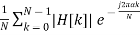
The FIR coefficient h[n] is calculated by IDFT of frequency samples.
h[n] = 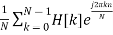 0≤k≤N-1.
=

= 
h[n] = 
α = [N-1]/2
For N=odd, summation limit will be [N-1]/2
Recursive frequency sampling filter
The recursive force of frequency sampling filter offers significant computational advantages over non recursive form if large number of frequency samples are zero valued. The transfer function of an FIR filter H[z] should be in recursive form. Impulse response of filter may be defined in terms of frequency samples.
h[n]= 
H[z]= 
Substituting value of h[n] and inter changing summation we have
H[z] = 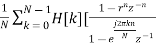 ]
]
H[z] can be represented as H[z] =H1[z]H2[z]
H1[z]=
H2[z] = 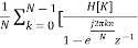 ]
]
Expanding above terms and solving them we finally get
H[z] = H1[z]H2[z]
H[z] = [
[
For frequency response we can replace z=ejωTs
H[ωn] = H[k] 0≤k≤N-1.
Q16) Draw block diagram for the function using parallel form H(z)=
A16)
H(z)=
Writing above transfer function in standard form for parallel realisation we get
H(z)=-20+
The structure is shown below
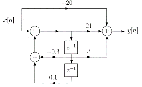
Fig: Parallel Realisation of H(z)=
Q17) For the following LTI system H(z)= . Realise the cascade form IIR filter.
A17) H(z)=
The above function can be simplified as
H(z)=

Fig: Cascade IIR Form
Hence, using the above structure and placing the values of 
 …. And similarly,
Q18) For the system given y(n) - y(n-1) +
  y(n-2) = x(n) +
  x(n-1) realises using cascade form?
A18) The system transfer function is given as
H(z) = Y(z)/X(z)
Taking z transform of y(n) - y(n-1) +
  y(n-2) = x(n) +
  x(n-1)
Y(z) -  z-1Y(z) +
  z-2 Y(z) = X(z) +
  z-1 X(z)
H(z)= 
Again, simplifying the above function to get into standard cascade form we ca write
H(z) = 
= H1(z)+H2(z)
H1(z)= 
H2(z)= 
The final structure is shown below

Fig: Cascade Form of H(z) = 
Q19) For the following LTI system H(z)= . Realise the cascade form?
A19) H(z)=
Writing the above in standard form for cascade realisation
H1(z)= 
H2(z)= 
The cascade structure is shown below
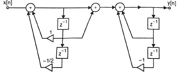
Fig: Cascade Form of H(z)=
Q20) Realize the system transfer function using parallel structure H(z)= 
A20) H(z)= 
Taking Z common and then dividing the above function to convert it into standard form for parallel realisation we get
H(z)=Z [  +
+ +
+ ]
]
The parallel structure is shown below
Fig: Parallel Realisation of H(z)= 
Q21) Realize the system transfer function using parallel structure H(z)= 
A21) Converting the above function to standard form using partial fraction technique
H(z)=  +
+ 
Solving for A and B we get
A= 10/3
B= -7/3
H(z) =  +
+ 
H1(z) = 
H2(z) = 
The parallel form realisation is shown below

Fig: Parallel Realisation of H(z)= 
Q22) For the transfer function H(z) =  . Realise using cascade form?
A22) H(z) = 
Writing in standard form
H(z) = 
H1(z) = 
H2(z) = 
The cascade structure is shown below

Fig: Cascade Form of H(z) = 


