Unit - 5
Analog Filters
Q1) Compare Impulse invariant and bilinear transformation filter design methods?
A1)
Sr No. | Impulse Invariance | Bilinear Transformation |
1 | In this method IIR filters are designed having a unit sample response h (n) that is sampled version of the impulse response of the analog filter. | This method of IIR filter design is based on the trapezoidal formula for numerical integration. |
2 | The bilinear transformation is a conformal mapping that transforms the j | The bilinear transformation is a conformal mapping tjat transforms the |
3 | For design of LPF, HPF and almost all types of bandpass and band stop filters, this method is used. | For designing of LPF, HPF and almost all types of bandpass and band stop filters, this method is used. |
4 | Frequency relationship is non –linear. Frequency warping or frequency compression is due to non – linearity. | Frequency relationship is nonlinear. Frequency warping or frequency compression is due to non – linearity. |
5 | All poles are mapped from s plane to the z plane by the relationship | All poles and zeros are mapped. |


Q2) Explain frequency wrapping in IIR filters?
A2) Frequency warping
• The bilinear transformation method has the following important features: A stable analog filter gives a stable digital filter. The maxima and minima of the amplitude response in the analog filter are preserved in the digital filter. As a consequence, – the pass band ripple, and – the minimum stop band attenuation of the analog filter are preserved in the digital filter frame.
• To determine the frequency response of a continuous-time filter, the transfer function Ha(s)Ha(s) is evaluated at s=jω which is on the jω axis. Likewise, to determine the frequency response of a discrete-time filter, the transfer function Hd(z) is evaluated at z=ejωT which is on the unit circle, |z|=1|z|=1 .
• When the actual frequency of ω is input to the discrete-time filter designed by use of the bilinear transform, it is desired to know at what frequency, ωa , for the continuous-time filter that this ω is mapped to.


• This shows that every point on the unit circle in the discrete-time filter z-plane, z= ejωT is mapped to a point on the jω axis on the continuous-time filter s-plane, s=jω. That is, the discrete-time to continuous-time frequency mapping of the bilinear transform is
ωa=(2/T) tan(ωt/2)
and the inverse mapping is
ω=(2/T) arc tan(ωaT/2)
• The discrete-time filter behaves at frequency the same way that the continuous-time filter behaves at frequency (2/T)tan(ωT/2). Specifically, the gain and phase shift that the discrete-time filter has at frequency ω is the same gain and phase shift that the continuous-time filter has at frequency (2/T)tan(ωT/2). This means that every feature, every "bump" that is visible in the frequency response of the continuous-time filter is also visible in the discrete-time filter, but at a different frequency. For low frequencies (that is, when ω≪2/T or ωa≪2/T),ω≈ωa.
One can see that the entire continuous frequency range
−∞<ωa<+∞
is mapped onto the fundamental frequency interval
−πT<ω<+πTω=±π/T.ωa=±∞
One can also see that there is a nonlinear relationship between ωa and ω This effect of the bilinear transform is called frequency warping.

Fig 1 Frequency wrapping
Q3) Design a discrete time lowpass filter to satisfy the following amplitude specifications: 

A3) Assume 
The pre-warped critical frequency are


Since both the passband and stopband are required to be monotonic, a Butterworth approximation will be used


From the Butterworth design tables we can immediately write

Now find H (z) by first noting that 


Using the pole/ zero mapping formula


We can now write

Find  by setting


Finally, after multiplying out the numerator and denominator we obtain

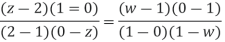
Q4) Find the bilinear transformation which maps points z =2,1,0 onto the points w=1,0,i.
Ans. Let, 
And, 
Since bilinear transformation preserves cross ratios,
Thus we have,


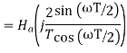
Use the bilinear transformation to convert the analog filtrt with system function

 into a digital IIR filter. Select T =0.1
Consider the following system function

Note that the following is the resonant frequency of the analog filter

Consider that the resonant frequency of analog filter must be mapped by selecting the value of parameter
T= 0,1
Use the following mapping for bilinear transformation

Write the system function H(z) of the resultant digital filter

Q5) Explain transversal structure of FIR adaptive filters?
A5) Transversal Structure Figure below shows the structure of a transversal FIR filter with N tap weights (adjustable during the adaptation process) with values at time n denoted as w0(n), w1 (n), ..., wN – 1(n). The tap-weight vector, w(n), is represented as
w(n) = [w0(n) w1(n) ... wN-1(n)] T
The tap-input vector, u(n), as
u(n) = [u(n) u(n-1) ... u(n-N+1)] T
The FIR filter output, y(n), can then be expressed as
y(n) = wT(n) u(n) = 
Where T denotes transpose, n is the time index and N is the order of the filter.

Fig 2 Transversal FIR Filter Structure
Q6) Explain symmetric transversal structure for adaptive filters?
A6) The characteristic of linear phase response in a filter is sometimes desirable because it allows a system to reject or shape energy bands of the spectrum and still maintain the basic pulse integrity with a constant filter group delay. Imaging and digital communications are examples of applications where this characteristic is desirable. An FIR filter with time domain symmetry, such as
w0(n) = wN – 1(n), w1(n) = wN - 2(n)... has a linear phase response in the frequency domain.
Consequently, the number of weights is reduced by a half in a transversal structure, as shown in Figure below with an even N tap weight. The tap-input vector becomes
u(n) = [u(n) + u(n – N +1 ), u(n – 1) + u(n – N + 2), ... ,u(n – N/2 + 1) + u(n - N/2)] T
As a result, the filter output y(n) becomes
y(n) = 

Fig 3 Symmetric Transversal Filter Structure
Q7) Explain the lattice structure for FIR adaptive filters?
A7) The lattice filter has a modular structure with cascaded identical stages. Figure shows one stage of a lattice FIR structure.

Fig 4 Lattice Structure
The lattice structure offers several advantages over the transversal structure:
• The lattice structure has good numerical round-off characteristics that make it less sensitive than the transversal structure to round-off errors and parameter variations.
• The lattice structure orthogonalizes the input signal stage-by-stage, which leads to fast convergence and efficient tracking capabilities when used in an adaptive environment.
• The various stages are decoupled from each other, so it is relatively easy to increase the prediction order if required.
• The lattice filter (predictor) can be interpreted as wave propagation in a stratified medium. This can represent an acoustical tube model of the human vocal tract, which is extremely useful in digital speech processing. These advantages, however, come at the expense of an increased number of multiplies and adds for a given transfer function realization.
The following equations represent the dynamics of the mth stage of an order M lattice structure as derived from Figure above:
fm(n)=fm – 1(n) – Km(n) bm – 1(n – 1), 0 < M
bm(n)=bm – 1(n – 1) Km(n) fm – 1(n), 0 < m < M
where fm(n) represents the forward prediction error, bm(n) represents the backward prediction error, Km(n) is the reflection coefficient, m is the stage index, and M is the number of cascaded stages. Km(n) has a magnitude less than one.
The terms fm(n) and bm(n) are initialized as f0(n) = b0(n) = u(n) where u(n) is the input signal. Speech analysis is usually performed by using the lattice structure and the reflection coefficients Km(n). Since the dynamic range of Km(n) is significantly smaller than that of the tap weights, w(n), of a transversal filter, the reflection coefficients require fewer bits to represent them. Hence, Km(n) are transmitted over the channel.
Q8) Explain LMS adaptive filter algorithm?
A8) The LMS Algorithm is initialized by setting all the weights to zero at time n=0. Tap weights are updated using the relationship
w(n+1) = w(n) + µe(n)u(n)
where w(n) represents the tap weights of the transversal filter, e(n) is the error signal, u(n) represents the tap inputs, and the factor µ is the adaptation parameter or step-size. To ensure convergence, µ must satisfy the condition
0 < µ < (2 / total input power)
where the total input power refers to the sum of the mean-square values of the tap inputs u(n), u(n-1), ..., u(n-N+1). Moreover, the LMS convergence time depends on the ratio of maximum to minimum eigenvalues of the autocorrelation matrix R of the input signal. To insure, that µ does not become sufficiently large to cause filter instability, a Normalized LMS algorithm can be employed. The normalized LMS employs a time-varying mu defined as
mu=x/uT(n).u(n)
where x is the normalized step-size chosen between 0 and 2. Tap weights are updated according to the relationship
w(n+1) = w(n) +xe(n)u(n)/[r+uT(n)u(n)]
The term x is the new normalized adaptation constant, while r is a small positive term included to ensure that the update term does not become excessively large when uT(n)u(n) temporarily becomes small. A problem can occur when the autocorrelation matrix associated with the input process has one or more zero eigenvalues. In this case, the adaptive filter will not converge to a unique solution. In addition, some uncoupled coefficients (weights) may grow without bound until hardware overflow or underflow occurs. This problem can be remedied by using coefficient leakage. This “leaky” LMS algorithm can be written as
w(n+1) = (1-µr )w(n) + µe(n)u(n)
where the adaptation constant µ and the leakage coefficient r are a small-positive values.
Q9) Explain the RLS adaptive filter algorithm?
A9) The LMS algorithm has many advantages (due to its computational simplicity), but its convergence rate is slow. The LMS algorithm has only one adjustable parameter that affects convergence rate, the step-size parameter µ, which has a limited range of adjustment in order to insure stability.
For faster rates of convergence, more complex algorithms with additional parameters must be used. The RLS algorithm uses a least-squares method to estimate correlation directly from the input data. The LMS algorithm uses the statistical mean-squared-error method, which is slower. The RLS algorithm uses a transversal FIR filter implementation. The order of operations the algorithm takes is
1. Compute the filter output (tap weights initialized to zero)
2. Find the error signal
3. Compute the Kalman Gain Vector (defined below)
4. Update the inverse of the correlation matrix
5. Update the tap weights
The Kalman Gain Vector is based on input-data autocorrelation results, the input data itself, and a factor called the forgetting factor. The forgetting factor ranges between zero and one and provides a time-weighting of the input data such that the most recent data points are weighted more heavily than past data. This allows the filter coefficients to adapt to time varying statistical characteristics of the input data. The tap weight update is based on the error signal and the Kalman Gain Vector and is expressed as
w(n) = w(n-1) + Ke(n)
where K is the Kalman Gain Vector and e(n) represents the error signal.
Q10) Write matlab program for DFT without function?
A10) % DFT program without function
clc;
close all;
clear all;
x=input('Enter the sequence x= ');
N=input('Enter the length of the DFT N= ');
len=length(x);
if N>len
x=[x zeros(1,N-len)];
elseif N<len
x=x(1:N);
end
i=sqrt(-1);
w=exp(-i*2*pi/N);
n=0:(N-1);
k=0:(N-1);
nk=n'*k;
W=w.^nk;
X=x*W;
disp(X);
subplot(211);
stem(k,abs(X));
title('Magnitude Spectrum');
xlabel('Discrete frequency');
ylabel('Amplitude');
grid on;
subplot(212);
stem(k,angle(X));
title('Phase Spectrum');
xlabel('Discrete frequency');
ylabel('Phase Angle');
grid on;
Output
Enter the sequence x= [4 5 6 9]
Enter the length of the DFT N= 7
Columns 1 through 4
24.0000 -2.3264 -13.6637i 3.0930 + 4.7651i
1.2334 - 6.2528i
Columns 5 through 7
1.2334 + 6.2528i 3.0930 - 4.7651i -2.3264 +13.6637i
Output

Q11) Determine the Fourier transform of the following sequence. Use the FFT (Fast Fourier Transform) function, using inbuilt function x (n) = {4 6 2 1 7 4 8}
A11) MATLAB Code:
% for defined sequence using inbuilt function
n = 0:6;
x = [4 6 2 1 7 4 8];
a = fft(x);
mag = abs(a);
pha = angle(a);
subplot(2,1,1);
plot(mag);
grid on
title('Magnitude Response');
subplot(2,1,2);
plot(pha);
grid on
title('phase Response');
Q12) Implementation of FFT of given sequence in matlab n-point FFT without in-built function?
A12) clear all;
close all;
clc;
x=input('Enter the sequence x[n]= ');
N=input('Enter the value N point= ');
L=length(x);
x_n=[x,zeros(1,N-L)];
for i=1:N
for j=1:N
temp=-2*pi*(i-1)*(j-1)/N;
DFT_mat(i,j)=exp(complex(0,temp));
end
end
X_k=DFT_mat*x_n';
disp('N point DFT is X[k] = ');
disp(X_k);
mag=abs(X_k);
phase=angle(X_k)*180/pi;
subplot(2,1,1);
stem(mag);
xlabel('frequency index k');
ylabel('Magnitude of X[k]');
axis([0 N+1 -2 max(mag)+2]);
subplot(2,1,2);
stem(phase);
xlabel('frequency index k');
ylabel('Phase of X[k]');
axis([0 N+1 -180 180]);
Q13) Write FFT matlab code for user defined sequence?
A13) %fast fourier transform
clc;
clear all;
close all;
tic;
x=input('enter the sequence');
n=input('enter the length of fft'); %compute fft
disp('fourier transformed signal');
X=fft(x,n)
subplot(1,2,1);stem(x); title('i/p signal');
xlabel('n --->');
ylabel('x(n) -->');grid;
subplot(1,2,2);stem(X);
title('fft of i/p x(n) is:');
xlabel('Real axis --->');
ylabel('Imaginary axis -->');grid;
OUTPUT
enter the sequence[1 .25 .3 4]
enter the length of fft4
fourier transformed signal
X =
5.5500 0.7000 + 3.7500i -2.9500 0.7000 - 3.7500i
Graph output

Q14) Write code for Z transform of an, 1+n and IZT of an?
A14) clc ;
close all;
syms n;
a=2;
x=a^n;
X=ztrans(x); %finding z transform
disp('z tranform of a^n a>1');
disp(X);
syms n;
a=0.5;
x=a^n;
X1=ztrans(x);
disp('z tranform of a^n 0<a<1');
disp(X1);
syms n;
a=2;
x=1+n;
X2=ztrans(x);
disp('z tranform of 1+n');
disp(X2);
A=iztrans(X);
disp('inverse z tranform of a^n a>1');
disp(A);
B=iztrans(X1);
disp('inverse z tranform of a^n 0<a<1');
disp(B);
C=iztrans(X2);
disp('inverse z tranform of 1+n');
disp(C);
subplot(1,3,1);
zplane([1 0],[1 -2]);
subplot(1,3,2);
zplane([1 0],[1 -1/2]);
subplot(1,3,3);
zplane([1 0 0],[1 -2 1]);
OUTPUT:
z tranform of a^n 0<a<1
z/(z - 1/2)
z tranform of 1+n
z/(z - 1) + z/(z - 1)^2
inverse z tranform of a^n a>1
2^n
inverse z tranform of a^n 0<a<1
(1/2)^n
inverse z tranform of 1+n
n + 1
Figure

Q15) Using matlab convert the following continuous time system to a discrete time system using a sampling time of 0.1.
H(s) = (s+2)/(s2+3s+2)
Code
num=[1 2];
den= [1 3 2];
sys=tf(num,den)
sys2=c2d(sys,0.1)
step(sys)
hold on step(sys2)
Output
For continuous system (s+2)/(s2+3s+2)
For discrete time system (0.095z-0.077)/(z2-1.724z+0.7408)
Q16) Find IZT of F(z)=z/z-0.5
A16) Code
syms z k
F=z/(z-0.5);
a=iztrans(F,k)
pretty(a)
Output
a= (0.5) k


