A1) Using the design formula for N N = [2.08]=3 Note: The normalized system function is
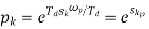
With poles at
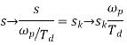
To frequency scale
So in the z domain
Note that when the design originates from discrete time specifications the poles of H (z) are independent of |
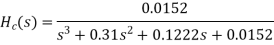


A2) First order transfer function of LPF is Step 1: HL(s) = Step 2: Prewrap critical frequency Ωp = tan(ωp Ts/2)= tan[(30x2xπ)/(2x150)] =0.7265 Step 3: Using LPF to HPF Transformation equation HH(s) = HL(s) = For LPF HH(s) =
|


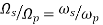
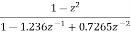
A3) STEP 1: Passband edge frequency ω1 =200Hz ω2= 300Hz STEP 2: Prewrap critical frequency Ω1 = tan(ω1 Ts/2)= tan(200xπ/2000) = 0.3249 Ω2 = tan(ω2 Ts/2)= tan(300xπ/2000) = 0.5095 STEP 3: W = Ω2 – Ω1 = 0.5095-0.3249 = 0.1846 STEP 4:HB(s) = HL(s) for s = S= For LPF HB(s) = STEP 5: Replace s by HB(s) = H(z) = 0.1367 [
|


A4)
|
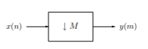
A5) Decimation, or down-sampling, consists of reducing the sampling rate by a factor M, cf. Figure 2.1. Here, the output is defined as
Fig 1 Decimation by factor M
y(m) = x(mM) i.e., it consists of every Mth element of the input signal. It is clear that the decimated signal y does not in general contain all information about the original signal x. Therefore, decimation is usually applied in filter banks and preceded by filters which extract the relevant frequency bands. In order to analyze the frequency domain characteristics of a multirate processing system with decimation, we need to study the relation between the Fourier transforms, or the z-transforms, of the signals x and y. For simplicity we consider the case M = 2 only. Then the decimated signal y is given by y(m) = x(2m)
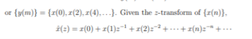
z-transform of y(m) is given by
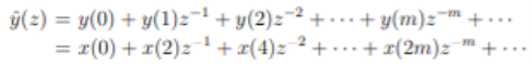
For finding the z-transform of y decimation is done in two stages as shown below
The above signal has z-transform as
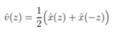
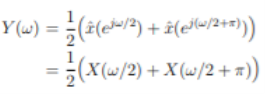
The Fourier transform of the decimated signal y(m) is related to z-transform by
But
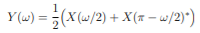
where X is the Fourier-transform of the sequence {x(n)}. But from the properties of the Fourier transform (periodicity and symmetry) it follows that X(ω/2 + π) = X(ω/2 − π) = X(π − ω/2)∗ . Hence
The Fourier-transform of {y(m)} thus cannot distinguish between the frequencies ω/2 and π − ω/2 of {x(n)}. This is equivalent to the frequency folding phenomenon occurring when sampling a continuous-time signal. Hence, whereas the signal {x(n)} consists of frequencies in [0, π], the frequency contents of the decimated signal {y(m)} are restricted to the range [0, π/2]. Moreover, after decimation of the signal {x(n)}, its frequency components in [0, π/2] cannot be distinguished from the frequency components in the range [π/2, π]. |


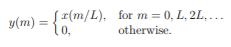
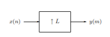
A6) Expansion, or up-sampling, consists of increasing the sampling rate by a factor L, cf. Figure below. Here, the output is obtained by inserting L-1 zeros between successive values of the input x(n)
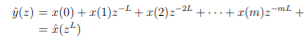
Fig 2 Interpolation by factor L The expansion operation followed by interpolation leads to a representation of the signal x at a sampling rate increased by the factor L. The expanded signal {y(m)} has the z-transform
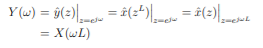
The Fourier Transform is
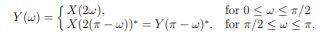
The transform Y (ω) at a given frequency ω ∈ [0, π] is thus equal to X(ωL), where ωL ∈ [0, Lπ]. But as the Fourier-transform is periodic with period 2π, we have X(ωL) = X(ωL + 2πk) = X((ω + 2πk L )L), and it follows that Y (ω) = Y (ω + 2πk L ). Hence Y (ω) is periodic, with L repetitions of X(ω) in the frequency range [0, 2π]. For example, for L = 2, we have X(2ω) = X(2ω − 2π) = X(2π − 2ω) ∗ = X(2(π − ω))∗ . Hence, for L = 2,
and Y (ω) is therefore uniquely defined by its values in the frequency band [0, π/2]. In order to reconstruct the correct interpolating signal at the higher sampling rate, an interpolating filter has to be introduced after the expansion. This is equivalent to the situation in D/A conversion, where a low-pass filter is used after the hold function. |
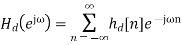
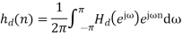
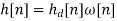
A7) Let the frequency response of the desired LTI ststem we wish to approximate be given by
Where Consider obtaining a casual FIR filter that approximates
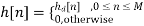
the FIR filter then has frequency response
Note that sibce we can write
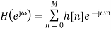
We are actually forming a finite Fourier series approximation to Since the ideal To allow for a less abrupt Fourier series truncation and hence reduce Gibbs phenomenon oscillations, we may generalize h [n] by writing
where |


A8) The Parks–McClellan Algorithm may be restated as the following steps:
To gain a basic understanding of the Parks–McClellan Algorithm mentioned above, we can rewrite the algorithm above in a simpler form as:
|
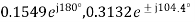
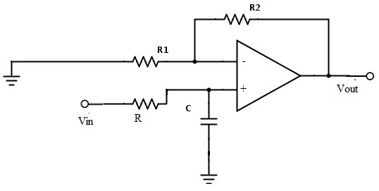
A9) The below circuit shows the low pass Butterworth filter:
Fig 3 First order LP Butterworth Filter
The required pass band gain of the Butterworth filter will mainly depends on the resistor values of ‘R1’ and ‘Rf’ and the cut off frequency of the filter will depend on R and C elements in the above circuit. The gain of the filter is given as Amax = 1 + (R1 / Rf) The impedance of the capacitor ‘C’ is given by the -jXC and the voltage across the capacitor is given as, Vc = - jXC / (R - jXC) * Vin Where XC = 1 / (2πfc), capacitive Reactance. The transfer function of the filter in polar form is given as H(jω) = |Vout/Vin| ∟ø Where gain of the filter Vout / Vin = Amax / √{1 + (f/fH)²} And phase angle Ø = - tan-1 ( f/fH ) At lower frequencies means when the operating frequency is lower than the cut-off frequency, the pass band gain is equal to maximum gain. Vout / Vin = Amax i.e. constant. At higher frequencies means when the operating frequency is higher than the cut-off frequency, then the gain is less than the maximum gain. Vout / Vin < Amax When operating frequency is equal to the cut-off frequency the transfer function is equal to Amax /√2. The rate of decrease in the gain is 20dB/decade or 6dB/octave and can be represented in the response slope as -20dB/decade. |
A10) Let us consider the Butterworth low pass filter with cut-off frequency 15.9 kHz and with the pass band gain 1.5 and capacitor C = 0.001µF. fc = 1/2πRC 15.9 * 10³ = 1 / {2πR1 * 0.001 * 10-6} R = 10kΩ Amax = 1.5 and assume R1 as 10 kΩ Amax = 1 + {Rf / R1} Rf = 5 kΩ
|