Unit-6
Numerical solution of Transcendental Equations, System of Linear equations and Expansion of Functions.
There are two types of equations Linear and Non linear equations. Linear equations are those in which dependent variable y is directly proportional to independent variable x and is of degree one. On the other hand non linear equation are those in which y does not directly proportional to x and of degree more than one.
Ex:  +b, where a and b are constant is a linear equation.
 is a non linear equation.


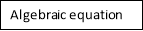
Algebraic Equation: If f(x) is a pure polynomial, then the equation  is called an algebraic equation in x.
Ex: 
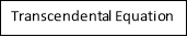
Transcendental Equation: If f(x) is an expression contain function as trigonometric, exponential and logarithmic etc. Then  is called transcendental equation.
Ex 
Non –linear equation can be solved by using various analytical methods. The transcendental equations and higher order algebraic equations are difficult to solve even sometime are impossible. Finding solution of equation means just to calculate its roots.
Numerical methods are often repetitive in nature. They consist of repetitive calculation of the same process; where in each step the result of preceding values are used (substitute). This is known as iteration process and is repeated till the result is obtained to desired accuracy.
The analytical methods used to solve equation; exact value of the root is obtained whereas in numerical method approximate value is obtained.
The numerical methods to find roots of non linear equations are:
- Regula-Falsi Method (Method of False position)
- Newton Raphson Method
Some important theorem:
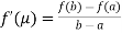
Theorem1: If f(x) is continuous in  ,and if f(a) anf f(b) are of opposite signs, then
  for atleast one numberµ such that
Theorem2:(Rolle’s theorem) If f(x) is continuous in  , f’(x) exists in
  and f(a) = f(b)=0 , then there exist one numberµ such that
  such that
Theorem3: (Intermediate value theorem) let f(x) be a continuous function in [a,b] and let k be any number between f(a) and f(b). Then there exists a µ in(a,b) such that f(µ) = k.
Theorem 4: (Mean Value theorem) Let f(x) be continuous in [a,b] and f’(x) exist in (a,b), then there exists at least one value of x, say µ, between a and b such that
6.1.1. Regula Falsi Method:
This is the oldest method of finding the approximate numerical value of a real root of an equation .
.
In this method we suppose that  and
and  are two points where
  and
and  are of opposite sign .Let
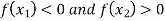
Hence the root of the equation  lies between
  and
and  and so,
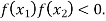
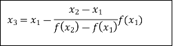
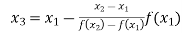
The Regula Falsi formula
Find  is positive or negative. If
  then root lies between
  and
and  or if
or if  then root lies between
  and
and  similarly we calculate
Proceed in this manner until the desired accurate root is found.
Example1 Find a real root of the equation 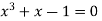 near
near , correct to three decimal place by the Regula Falsi method.
Let 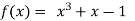
Now, 
And also 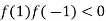
Hence the root of the equation  lies between
  and
and  and so,
By Regula Falsi Method

Now, 
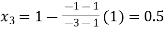
So the root of the equation  lies between 1 and 0.5 and so
By Regula Fasli Method

Now, 
So the root of the equation  lies between 1 and 0.63637 and so
By Regula Fasli Method

Now, 
So the root of the equation  lies between 1 and 0.67112 and so
By Regula Fasli Method

Now, 
So the root of the equation  lies between 1 and 0.63636 and so
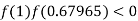
By Regula Fasli Method

Now, 
So the root of the equation  lies between 1 and 0.68168 and so
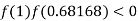
By Regula Fasli Method

Now, 
Hence the approximate root of the given equation near to 1 is 0.68217
Example2 Find the real root of the equation
By the method of false position correct to four decimal places
Let 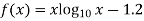
By hit and trail method

 0.23136 > 0
So, the root of the equation  lies between
  2 and
2 and  3 and also
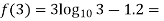
By Regula Falsi Mehtod


Now, 
So, root of the equation  lies between 2.72101 and 3 and also
By Regula Falsi Mehtod

Now, 
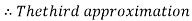
So, root of the equation  lies between 2.74020 and 3 and also
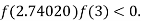
By Regula Falsi Mehtod

Now, 
So, root of the equation  lies between 2.74063 and 3 and also
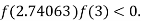
By Regula Falsi Mehtod
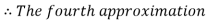

Hence the root of the given equation correct to four decimal places is 2.7406
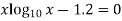
Example3 Apply Regula Falsi Method to solve the equation
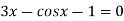
Let 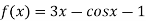
By hit and trail

And 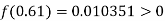
So the root of the equation lies between 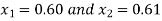 and also
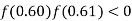
By Regula Falsi Mehtod


Now, 
So, root of the equation  lies between 0.60709 and 0.61 and also
By Regula Falsi Method


Now, 
So, root of the equation  lies between 0.60710 and 0.61 and also
By Regula Falsi Method

Hence the root of the given equation correct to five decimal place is 0.60710.
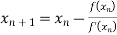
6.1.2. Newton-Raphson Method:
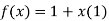
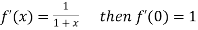
Let  be the approximate root of the equation
 .
.
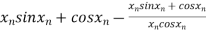
By Newton Raphson formula 
In general,
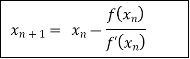
Where n=1, 2, 3…… we keep on calculating until we get desired root to the correct decimal places.
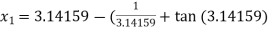
Example1 Using Newton-Raphson method, find a root of the following equation correct to 3 decimal places: .
.
Given 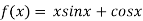
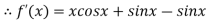

By Newton Raphson Method
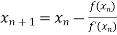
= 
=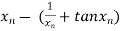
The initial approximation is 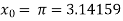 in radian.
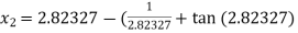
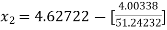
For n =0, the first approximation 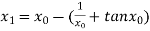

For n =1, the second approximation 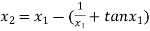

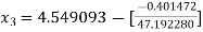
For n =2, the third approximation 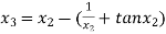
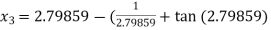

For n =3, the fourth approximation 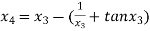
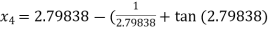
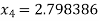
Hence the root of the given equation correct to five decimal place 2.79838.
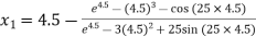
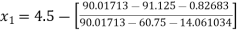
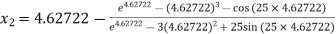
Example2 Using Newton-Raphson method, find a root of the following equation correct to 3 decimal places: 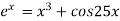 near to 4.5
Let 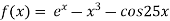

The initial approximation 
By Newton Raphson Method

For n =0, the first approximation 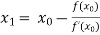
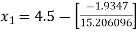

For n =1, the second approximation 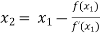
For n =2, the third approximation 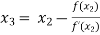

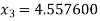
For n =3, the fourth approximation 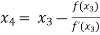

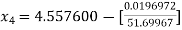

Hence the root of the equation correct to three decimal places is 4.5579
Example3 Using Newton-Raphson method, find a root of the following equation correct to 4 decimal places: 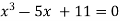
Let 

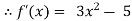
By Newton Raphson Method
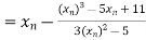

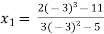
Let the initial approximation be 
For n=0, the first approximation 
For n=1, the second approximation 
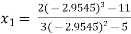

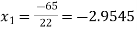
For n=2, the third approximation 
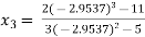

Since  therefore the root of the given equation correct to four decimal places is -2.9537
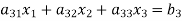
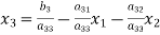
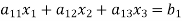
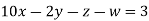
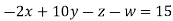
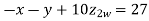
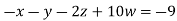
The standard a system of n linear equation in n unknown is 


 (1)
(1)
… …… …. …

6.2.1.Gauss Jacobi’s Iteration method :
Let us consider the system of simultaneous linear equation


 (1)
(1)
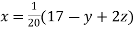
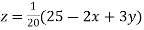
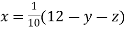
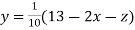
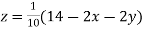
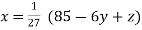
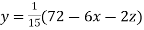
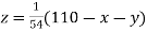
The coefficients of the diagonal elements are larger than the all other coefficients and are non zero. Rewrite the above equation we get


 (2)
(2)
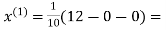
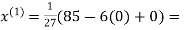
Take the initial approximation  we get the values of the first approximation of
 .
.
By the successive iteration we will get the desired the result.
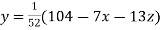
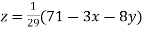
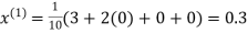
Example1Use Jacobi’s method to solve the system of equations:

Since 
So, we express the unknown with large coefficient in terms of other coefficients.

 (1)
(1)
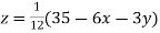
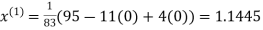
Let the initial approximation be 

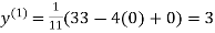
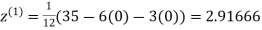


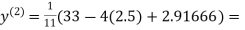 2.35606
 0.91666


 1.932936
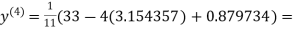
 0.831912

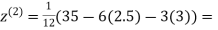
 3.016873
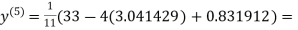 1.969654


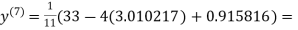
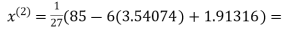
 3.010217
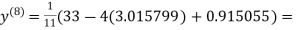
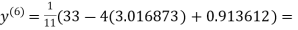 1.986010


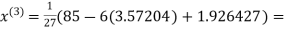
 1.988631
 0.915055


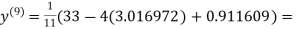
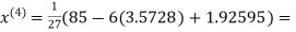
 1.986532
 0.911609


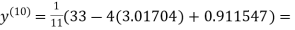
 1.985792
 0.911547


 1.98576
 0.911698
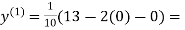
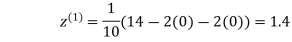
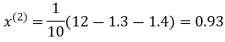
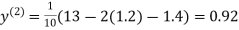
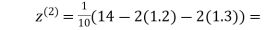
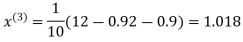
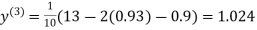
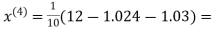
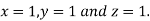
Since the approximation in ninth and tenth iteration is same up to three decimal places, hence the solution of the given equations is 
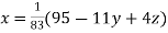
Example2 Solve by Jacobi’s Method, the equations

Given equation can be rewrite in the form
 … (i)
… (i)
 ..(ii)
 ..(iii)
Let the initial approximation be 

Putting these values on the right of the equation (i), (ii) and (iii) and so we get


Putting these values on the right of the equation (i), (ii) and (iii) and so we get


Putting these values on the right of the equation (i), (ii) and (iii) and so we get
 0.90025


Putting these values on the right of the equation (i), (ii) and (iii) and so we get


Putting these values on the right of the equation (i), (ii) and (iii) and so we get


Hence solution approximately is 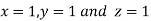
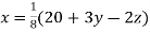
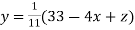
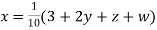
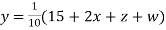
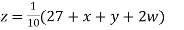
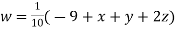
Example3Use Jacobi’s method to solve the system of the equations

Rewrite the given equations

 (1)
(1)
Let the initial approximation be 

 1.2
1.2
 1.3
1.3

 0.9
0.9

 1.03
1.03

 0.9946
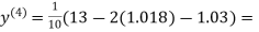 0.9934
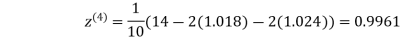

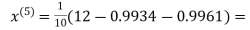 1.0015

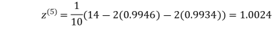
Hence the solution of the above equation correct to two decimal places is
6.3.1
6.2.3.Gauss Seidel method:
This is the modification of the Jacobi’s Iteration.
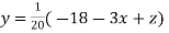
Let us consider the system of simultaneous linear equation

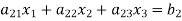 (1)
(1)

The coefficients of the diagonal elements are larger than the all other coefficients and are non zero. Rewrite the above equation we get


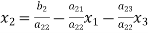 (2)
(2)

Take the initial approximation  we get the values of the first approximation of
 .
.
As above in Jacobi’s Iteration, we take first approximation as
 and put in the right hand side of the first equation of (2) and let the result be
  .
.
Now we put  right hand side of second equation of (2) and suppose the result is
Now put  in the RHS of third equation of (2) and suppose the result be
The above method is repeated till the values of all the unknown are found up to desired accuracy.
Example1 Use Gauss –Seidel Iteration method to solve the system of equations

Since 
So, we express the unknown of larger coefficient in terms of the unknowns with smaller coefficients.
Rewrite the above system of equations

 (1)
(1)
Let the initial approximation be 

 3.14814


 2.43217


 2.42571


 2.4260


Hence the solution correct to three decimal places is

Example2 Solve the following system of equations

By Gauss-Seidel method.
Rewrite the given system of equations as

 (1)
(1)
Le t the initial approximation be 


Thus the required solution is 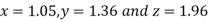
Example3 Solve the following equations by Gauss-Seidel Method
Rewrite the above system of equations

 (1)
(1)
Let the initial approximation be 


Hence the required solution is 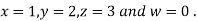
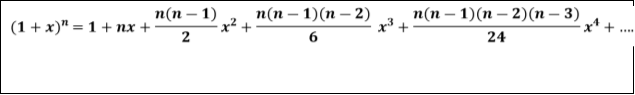
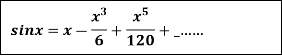
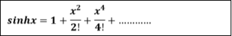
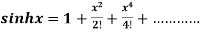
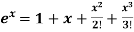
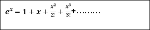
Expansion of some well known series:
a) 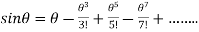
b) 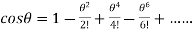
c) 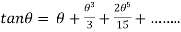
d) 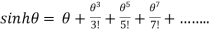
e) 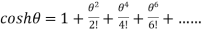
f) 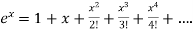
g) 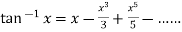
h) 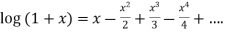
i) 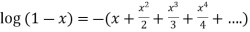
j) 
6.3.1Taylor’s theorem:
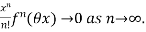
If (i) f(x) and its first (n-1) derivative be continuous in [a, a+h],
(ii)  exist for every value of x in (a, a+h), then there is at least one number
  such that

This is called Taylor’s theorem with Lagrange’s form of remainder


Taylor’s Series:
If  can be expanded as an infinite series, then

If  possesses derivative of all orders and the remainder
  .
.
Corollary: Taking  and
and  in equation (i) we get

Taking  in above we get Maclaurin’s series.
Example1: Expand the polynomial 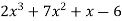 in power of
  , by Taylor’s theorem.
Let 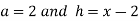 .
.
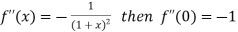
Also 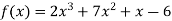
Then 
Differentiating with respect to x.
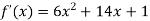
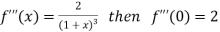
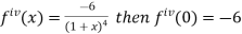
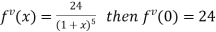
Again differentiating with respect to x the above function.
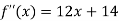
Again differentiating with respect to x the above function.

Also the value of above functions at x=2 will be


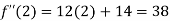

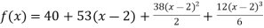
By Taylor’s theorem
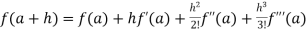
On substituting above values we get


Example2: Expand  in power of
Let 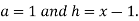
Also 
Differentiating f(x) with respect to x.

Again differentiating f(x) with respect to x.
Again differentiating f(x) with respect to x.
Also the value of above functions at x=1 will be
By Taylor’s theorem

On substituting above values we get


 =
= 
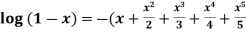
Example3: Expand  in power of
 . Hence find the value of
  correct to four decimal places.
Let 
And 
 .
.
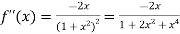
Differentiating  with respect to x.

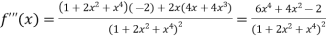
Again differentiating  with respect to x.

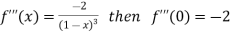
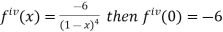
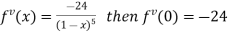
Again differentiating  with respect to x.
Again differentiating  with respect to x.

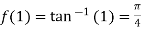
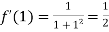
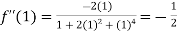
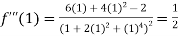
Also the value of above functions at  will be

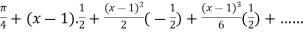
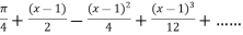
By Taylor’s theorem

On substituting above values we get
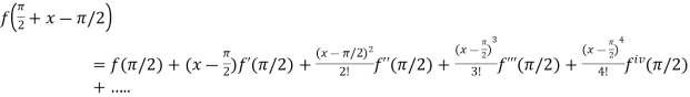
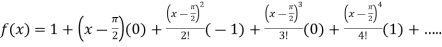
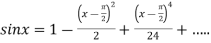
At 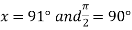

 .
.
6.3.2.Maclaurin’s theorem:
This is a particular case of Taylor’s theorem in which a=0 and h=x in Taylor’s theorem.
If f(x) can be expanded as an infinite series, then

Where the remainder is 
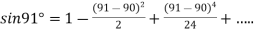
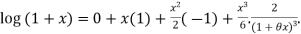
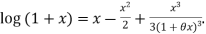
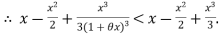
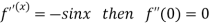
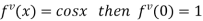
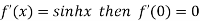
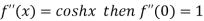
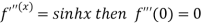
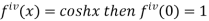
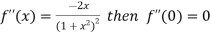
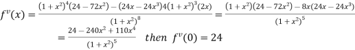
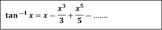
Example1:If 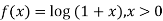 using Taylor’s theorem, show that for
  .
.

Deduce that 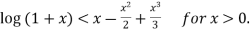
Let 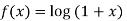 then
then 
Differentiating with respect to x.
 .Then
.Then 
Again differentiating with respect to x.
 Then
Then 
Again differentiating with respect to x.
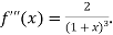 Then
Then 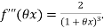
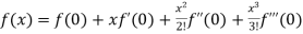
By Maclaurin’s theorem

Substituting the above values we get
Since 
Hence 
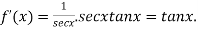
Example2: Prove that 
Let 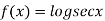
Differentiating  with respect to x.
Again differentiating  with respect to x.

Again differentiating  with respect to x.

Again differentiating  with respect to x.
 and so on.
Putting  , in above derivatives we get
 so on.
By Maclaurin’s theorem
 +………
+………
Substituting the above values we get

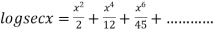
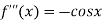
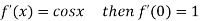
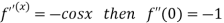
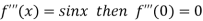
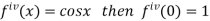
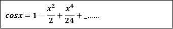
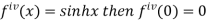
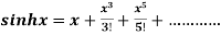
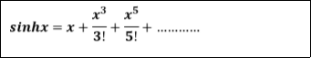
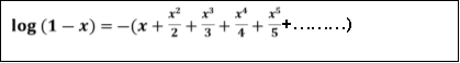
Example3: Prove that
Let 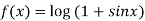
Differentiating above function with respect to x.
Again differentiating above function with respect to x.

Again differentiating above function with respect to x.
Again differentiating above function with respect to x.
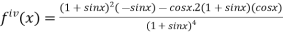
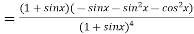
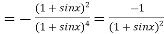
Putting  , in above derivatives we get
 so on.
By Maclaurin’s theorem
 +………
+………
Substituting the above values we get


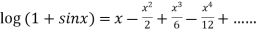
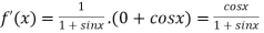
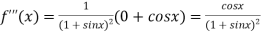
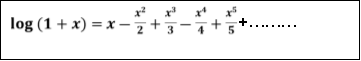
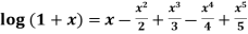
Example: Expansion of Some standard series

Let  and
and 
Differentiating above function with respect to x.


By Maclaurin’s theorem
 +………
+………
Substituting the above values we get

2. 
Let  and
and 
Differentiating above function with respect to x.

By Maclaurin’s theorem
 +………
+………
Substituting the above values we get


3.
Let  and
and 
Differentiating above function with respect to x.
 .
.


By Maclaurin’s theorem
 +………
+………
Substituting the above values we get

4. 
Let  and also
Differentiating above function with respect to x.


By Maclaurin’s theorem
 +………
+………
Substituting the above values we get

5. 
Let  and also
Differentiating above function with respect to x.

By Maclaurin’s theorem
 +………
+………
Substituting the above values we get

6. 
Let  and also
Differentiating above function with respect to x.


By Maclaurin’s theorem
 +………
+………
Substituting the above values we get


7. 
Let 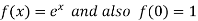
Differentiating above function with respect to x.
By Maclaurin’s theorem
 +………
+………
Substituting the above values we get
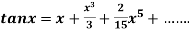
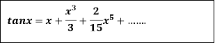
 +
+ +………
+………
 +………
+………
8. 
Let 
Differentiating above function with respect to x.
By Maclaurin’s theorem
 +………
+………
Substituting the above values we get
 +………
+………
 +………
+………
9. 
Let 
Differentiating above function with respect to x.
By Maclaurin’s theorem
 +………
+………
Substituting the above values we get
 +………
+………
 +………)
+………)
10. 
Let 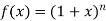
Differentiating the above function with respect to x.


By Maclaurin’s theorem
 +………
+………
Substituting the above values we get