Unit-5
Decision theory
Concept of decision making-
According to Haynes and Massie, “Decision making is a process of selection form a set of alternative courses of action which is thought to fulfil the objective of the decision problem more satisfactorily than others.”
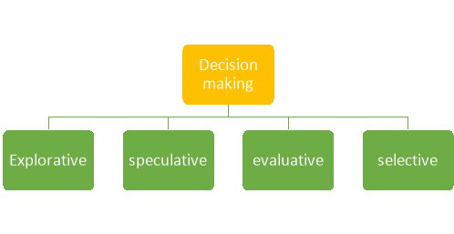
Decision making is the process of selection and aim is to select the best alternatives. There are four phases in this process- Explorative, speculative, evaluative and selective.
Decision theory deals with how to determine the best course of action when many options are available and the outcome cannot be reliably predicted.
It's hard to imagine a situation without such a decision problem, but we're primarily limited to problems that occur in the business, and the results can be explained in dollars of profit or revenue, cost or loss. It may be reasonable to consider these issue as the best alternative in the long run, with the highest profit or profit on average, or the lowest cost or loss. This criterion of optimality is not without its drawbacks, but it should serve as a useful guide to behavior in repetitive situations where the results are not critical. (Another criterion of optimality, maximizing expected usefulness, provides consistent decision makers with a more personal and subjective guide to behavior.)
The simplest decision problem is to list the probabilities associated with the possible monetary outcome of each alternative, calculate the expected monetary value of all alternatives, and select the alternative with the highest expected monetary value. You can solve it by doing. Determining the best alternative is a bit more complicated when:
The alternative involves a series of decisions.
Another class of problem often gets additional information about uncertain variables at a particular cost. This additional information is rarely completely accurate. Its value, and the maximum amount you are willing to pay to get it, must depend on the difference from the best you can expect to do with the help of this information.
And the best I expect to do without it. These are the types of problems we are about to start.
Decision making and problem solving are directly related with planning.
In the planning procedure, managers decide the goals to be persued, what kind of resources will be used and what steps will be taken to meet the target.
The quality of decision determines how effective the plan is.
Definition-
A decision may be defined as the selection of the action, by the decision maker, which is considered to be the best according to some predetermined standard from amongst the available options.
Steps in Decision making-
I) Identification of all possible outcomes called states of nature or events.
Ii) Identification of all courses of action called acts.
Iii) Determination of payoff function.
Iv) Choosing from among the alternatives, the best possible action on the basis of some criterion.
Characteristics of decision making
- Decision making is a goal-oriented process. Decisions are made to achieve certain goals.
- It involves choice. Or selection of the most appropriate course of action out of various alternatives.
- It is an ongoing process. Decision making is a recurring activity.
- It is a intellectual process. It involves intuitions and experience.
- It is a dynamic process. Technique used for decision making may vary with the type of problem involved and the time available for its solution.
- It is situational. There may also be a decision not to act.
- It involves commitment of time, efforts and resources.
- It is pervasive.
Key takeaways-
- Decision theory deals with how to determine the best course of action when many options are available and the outcome cannot be reliably predicted.
- A decision may be defined as the selection of the action, by the decision maker, which is considered to be the best according to some predetermined standard from amongst the available options.
- Decision making is a goal-oriented process. Decisions are made to achieve certain goals.
- Decision making is a dynamic process. Technique used for decision making may vary with the type of problem involved and the time available for its solution
Decision making iinvolves commitment of time, efforts and resources.
A payoff matrix is a table in which strategies of one player are listed in rows and those of the other player in columns and the cells show payoffs to each player such that the payoff of the row player is listed first.
A payoff matrix lists the name of the row player to the left of the matrix and the name of the column player above the matrix. The strategies of the row player form the rows of the matrix and the strategies of the column player form its column.
Example: Let us consider two companies: Row and Column. Currently, they share the market equally. There is a Rs. 20 Lakhs worth of untapped market. If Row expands its network, it will be able to capture the whole $50 million revenue if Column does not expand its network, and vice versa. Similarly, if both expand their network, Row will get $20 million additional revenue and Column $30 million, but if no one expands its network, both gets zero additional revenue.
Let us create a payoff matrix for this game.
- There are two players: Row and Column and each has two strategies i.e. to expand or not to expand. Hence, there must be four cells in the matrix.
- We list Row as the player whose strategies are listed in rows in red and Column as the player whose strategies are tabulated in columns in blue.
- The upper left cell corresponds a strategy in which both firms expand. In such an eventuality, Row gets $20 million (which appears first) and Column gets $30 million (which appears last).
- The lower left cell corresponds to a strategy when Row does not expand but Column expands. The payoff to Row and Column in this case is 0 and $50 million, respectively. This payoff reverses in the upper right corner which represents payoff when Row expands but Column does not.
- The lower right cell represents a situation in which neither firm moves to capture the market, and both get a payoff of zero.
The following table shows the different ways in which the payoff matrix may be presented.
State of nature-
“In decision theory, state of nature refer to the possible condition which may happen in the future.”
Key takeaways-
1. Payoff matrix is a table in which strategies of one player are listed in rows and those of the other player in columns and the cells show payoffs to each player such that the payoff of the row player is listed first
Decision making environment-
Making decisions is a integral part of manager’s work. A manager must make strategies as well as routine decisions.
While taking decision, manager should gather information related to the decision and check the various issues and outcomes related to the decision.
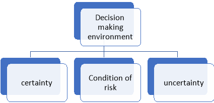
The decision making is categorized as-
- Certainty.
- Risk.
- Uncertainty.
Certainty- it is an environment of very low ambiguity. Under these conditions, the manager has complete and measurable info about the objectives, as well as outcomes of the alternative decisions. Certainty is an ideal situation where the manager has perfect info.
Another way to ensure a secure environment is for the manager to create a closed system. This means he chooses to focus on only a few options. He gets all the information available about such alternatives that he is analyzing. He ignores other factors that make the information unavailable. Such factors have nothing to do with him.
Risk- This is a condition of moderate ambiguity. Decision makers take decision in a risky environment. In this situation, the decision maker has incomplete info.
However, the possible outcomes can be assigned probability estimates. Probabilities may be derived from mathematical or statistical models.
In order to make good decisions decision makers must do systematic research and collect info. Related to outcomes.
Even in this scenario, the manager has some information available. However, the availability and reliability of the information is not guaranteed. He needs to graph some alternative behavioral policies from the data he has.
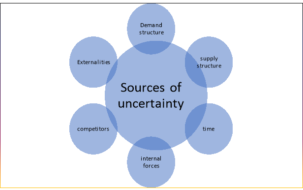
Uncertainty- Uncertainty is an integral element of future. Keynes in 1921 introduced the concept of uncertainty.
It is the condition of high ambiguity and unpredictability. It is associated with a very dynamic external environment and lack of availability of info.
In case of uncertainty, the decision maker does not have sufficient info to assign probabilities to the outcomes. Fuzzy logic can be used to take quantitative decisions. Non-mathematical techniques may also be used to take decision under uncertainty.
In an uncertain environment, everything is in flux. Some external and random forces mean that the environment is the most unpredictable.
In these chaotic times, all variables change rapidly. However, managers need to fully understand this mayhem. He must create some order, obtain reliable data, and make the best decisions according to his judgment.
Key takeaways-
- Certainty- it is an environment of very low ambiguity. Under these conditions, the manager has complete and measurable info about the objectives, as well as outcomes of the alternative decisions.
- Risk- This is a condition of moderate ambiguity. Decision makers take decision in a risky environment. In this situation, the decision maker has incomplete info.
However, the possible outcomes can be assigned probability estimates.
3. Uncertainty- Uncertainty is an integral element of future. Keynes in 1921 introduced the concept of uncertainty.
a) Maximax Criterion: In this case the decision maker does not want to miss the opportunity to achieve the largest possible profit.
Steps: 1) Locate the maximum Payoff values corresponding to each act.
2) From among the maximum choose the highest value.
This is also called the optimistic criterion because the decision maker chooses the best of the best
B) Maxima criterion: This is a conservative approach. Here the decision maker attempts in maximizing the minimum possible profits.
C) Minimax Regret criterion: The Minimax Regret Criterion is a technique used to make decisions under uncertainty. ... Under this Minimax Regret Criterion, the decision maker calculates the maximum opportunity loss values (or also known as regret) for each alternative, and then she chooses the decision that has the lowest maximum regret.
For example, suppose Geoffrey Rams bottom is faced with the following pay-off table. He has to choose how many salads to make in advance each day before he knows the actual demand.
- His choice is between 40, 50, 60 and 70 salads.
- The actual demand can also vary between 40, 50, 60 and 70 with the probabilities as shown in the table - e.g. P (demand = 40) is 0.1.
- The table then shows the profit or loss - for example, if he chooses to make 70 but demand is only 50, then he will make a loss of $60.
Daily supply | ||||||
Daily Demand |
| Probability | 40 salads | 50 salads | 60 salads | 70 salads |
40 salads | 0.10 | 80 | 0 | (80) | (160) | |
50 salads | 0.20 | 80 | 100 | 20 | (60) | |
60 salads | 0.40 | 80 | 100 | 120 | 40 | |
70 salads | 0.30 | 80 | 100 | 120 | 140 | |
The question is then which output level to choose.
Maximax
The Maximax rule involves selecting the alternative that maximises the maximum payoff available.
This approach would be suitable for an optimist, or 'risk-seeking' investor, who seeks to achieve the best results if the best happens. The manager who employs the Maximax criterion is assuming that whatever action is taken, the best will happen; he/she is a risk-taker. So, how many salads will Geoffrey decide to supply?
Looking at the payoff table, the highest maximum possible pay-off is ₹140. This happens if we make 70 salads and demand is also 70. Geoffrey should therefore decide to supply 70 salads every day.
Maximin
The maximin rule involves selecting the alternative that maximises the minimum pay-off achievable. The investor would look at the worst possible outcome at each supply level, and then selects the highest one of these. The decision maker therefore chooses the outcome which is guaranteed to minimise his losses. In the process, he loses out on the opportunity of making big profits.
This approach would be appropriate for a pessimist who seeks to achieve the best results if the worst happens.
So, how many salads will Geoffrey decide to supply? Looking at the payoff table,
- If we decide to supply 40 salads, the minimum pay-off is ₹80.
- If we decide to supply 50 salads, the minimum pay-off is ₹0.
- If we decide to supply 60 salads, the minimum pay-off is (80).
- If we decide to supply 70 salads, the minimum pay-off is (160).
The highest minimum payoff arises from supplying 40 salads. This ensures that the worst possible scenario still results in a gain of at least ₹80.
Minimax regret
The minimax regret strategy is the one that minimises the maximum regret. It is useful for a risk-neutral decision maker. Essentially, this is the technique for a 'sore loser' who does not wish to make the wrong decision.
'Regret' in this context is defined as the opportunity loss through having made the wrong decision.
To solve this a table showing the size of the regret needs to be constructed. This means we need to find the biggest pay-off for each demand row, then subtract all other numbers in this row from the largest number.
For example, if the demand is 40 salads, we will make a maximum profit of ₹80 if they all sell. If we had decided to supply 50 salads, we would achieve a nil profit. The difference or 'regret' between that nil profit and the maximum of ₹80 achievable for that row is ₹80.
Regrets can be tabulated as follows:
Daily supply | |||||
Daily Demand |
| 40 salads | 50 salads | 60 salads | 70 salads |
40 salads | 0 | ₹80 | ₹160 | ₹240 | |
50 salads | ₹20 | ₹0 | ₹80 | ₹160 | |
60 salads | ₹40 | ₹20 | ₹0 | ₹80 | |
70 salads | ₹60 | ₹40 | ₹20 | ₹0 | |
The maximum regrets for each choice are thus as follows (reading down the columns):
- If we decide to supply 40 salads, the maximum regret is ₹60.
- If we decide to supply 50 salads, the maximum regret is ₹80.
- If we decide to supply 60 salads, the maximum regret is ₹160.
- If we decide to supply 70 salads, the maximum regret is ₹240.
Key takeaways-
b) Maximax Criterion: In this case the decision maker does not want to miss the opportunity to achieve the largest possible profit.
c) Maxima criterion: This is a conservative approach. Here the decision maker attempts in maximizing the minimum possible profits.
d) Minimax Regret criterion: The Minimax Regret Criterion is a technique used to make decisions under uncertainty. ... Under this Minimax Regret Criterion,
Introduction
Game theory is a theoretical framework for imagining social situations between competing players. In some respects, game theory is the best decision of an independent competing actor in the science of strategy, or at least in a strategic setting. Let's look at some examples.
The major pioneers of game theory were the 1940s mathematician John von Neumann and the economist Oskar Morgenstern. Mathematician John Nash is considered by many to provide the first significant extension of the work of von Neumann and Morgenstern!
Basics of game theory
The focus of theory of games may be a game that acts as a model for an interactive situation between rational players. The key to game theory is that the rewards of one player depend on the strategy implemented by the other player. The game identifies the player's identity, preferences, available strategies, and how these strategies affect results. Depending on the model, various other requirements and assumptions may be required.
According to game theory, the actions and choices of all participants influence their outcomes!
Let's start with Nash equilibrium
Nash equilibrium is the result reached, which means that once achieved, the payoff cannot be increased by unilaterally changing decisions. You can also think of it as "no regrets" in the sense that once you make a decision, you will not regret a decision that takes into account the consequences.
In most cases, the Nash equilibrium is achieved over time. However, once the Nash equilibrium is reached, it does not deviate. After learning how to find the Nash equilibrium, let's see how unilateral movements affect the situation. Does it make sense? The Nash equilibrium is described as "no regrets" because it should not be. It is generally believed that there is multiple equilibrium in a game.
This mainly happens in games that have more complex elements than the two choices of two players. In a simultaneous game that repeats over time, one of these multiple equilibrium is reached after trial and error. This scenario of various overtime choices before reaching equilibrium is most often performed in the business world when two companies are deciding on prices for compatible products such as airfares and soft drinks. The impact of game theory on economics and business
Game theory has revolutionized economics by addressing the critical problems of previous mathematical economic models. Neoclassical economics, for example, struggled to understand the expectations of entrepreneurs and was unable to cope with imperfect competition. Game theory turned its attention to the market process itself from steady-state equilibrium.
In business, game theory is undoubtedly useful for modeling competing behaviour between economic agents. Enterprises often have several strategic options that affect their ability to achieve economic benefits. For example, companies may face dilemmas such as discontinuing existing products, starting new product development, lowering prices compared to competitors, or adopting new marketing strategies. Economists tend to use game theory to understand the behaviour of oligopolistic businesses. This helps predict the possible consequences of a company engaging in certain actions such as price fixing or collusion.
The limits of game theory
The biggest problem with game theory, like most other economic models, is that it relies on the assumption that people are selfish and rational actors who maximize utility. We are social beings who often cooperate at our own expense and consider the welfare of others! Game theory cannot explain the fact that depending on the social situation and who the player is, the situation may or may not be in Nash equilibrium.
Two -person zero sum game payoff matrix
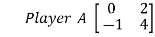
Determine which of the following two-person zero-sum games are strictly determinable and fair. Give optimum strategies for each player in the case of strictly determinable games:
(a) 
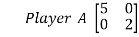
(b) 
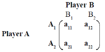
The payoff matrix for player A is
Player A | Player B | Row minima | |
B1 | B2 | ||
A1 | 5+ | 0* | 0 |
A2 | 0* | 2+ | 0 |
Column maxima | 5 | 2 |
|
The payoffs marked with [*] in each row reflect the minimum payoff and the payoffs marked with [+] in each column of the payoff matrix represent the full payoff.  (maximinim) is the largest portion of the minimum lines.
Value) and the smallest Column Maximum part represents  (minimax value).
Thus obviously, we have  =0 and
  2.
2.
Since 
 , the game is not strictly determinable.
Pure Strategy Games (Saddle Point available). Principles of Dominance method
Consider the example of solving a game whose pay-off matrix is given as follows in the following table:
Issue of the Game
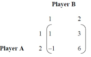
The game is worked out using the minimax method. In each row, find the smallest value and select the largest value from these values. Next, in each column, find the largest value and pick the smallest of these numbers. The following table shows the procedure.
Minimax Procedure
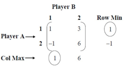
If Maximum value in row is equal to the minimum value in column, then saddle point exists.
Max Min = Min Max
1 = 1
Therefore, there is a saddle point.
The strategies are,
Player A plays Strategy A1, (A A1).
Player B plays Strategy B1, (B B1).
Value of game = 1.
Mixed strategies: Games without saddle point.
For any given pay off matrix without saddle point the optimum mixed strategies are shown in Table
Mixed Strategies
Let p1 and p2 be the probability for Player A.
Let q1 and q2 be the probability for Player B.
Let the optimal strategy be SA for player A and SB for player B.
Then the optimal strategies are given in the following tables.
Optimum Strategies
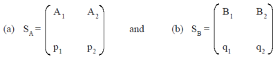
p1and p2 are determined by using the formulae,
p1 =
a22-a21
(a11+a22)-(a12+a21
And p2= 1-p1
q1=
a22-a21
(a11+a22)-(a12+a21
and q2= 1-q1
the value of the game w.r.t. Player A is given by,
Value of the game, v =
a11 a22– a12a21
(a11+a22)-(a12+a21
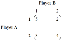
Example: Solve the pay-off given table matrix and determine the optimal strategies and the value of game.
Game Problem
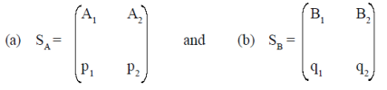
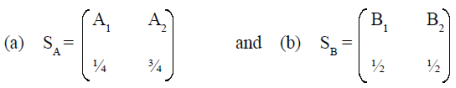
Solution: Let the optimal strategies of SA and SB is as shown in tables.
Optimal Strategies
The given pay-off matrix is shown below in Table.
Pay-off Matrix or Maximin Procedure
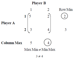
Therefore, there is no saddle point and hence it has a mixed strategy. Applying the probability formula,
p1 =
a22-a21
(a11+a22)-(a12+a21
=
4-3
(5+4)-(2+3)
=
1
9-5
=
1
4
And p2= 1-p1
= 1-1/4= 3/4
q1=
a22-a21
(a11+a22)-(a12+a21
4-2
(5+4)-(2+3)
=
2
9-5
=
1
2
And q2= 1-q1
Value of the game, v =
a11 a22– a12a21
(a11+a22)-(a12+a21
=14/4
The optimum mixed strategies are shown in table below.
Optimum Mixed Strategies
Key takeaway:
- Game theory is a theoretical framework for imagining social situations between competing players. In some respects, game theory is the best decision of an independent competing actor in the science of strategy, or at least in a strategic setting.
- The focus of theory of games may be a game that acts as a model for an interactive situation between rational players.
- The key to game theory is that the rewards of one player depend on the strategy implemented by the other player.
- Game theory has revolutionized economics by addressing the critical problems of previous mathematical economic models.
- The biggest problem with game theory, like most other economic models, is that it relies on the assumption that people are selfish and rational actors who maximize utility.
- The prisoner's dilemma was played once by two players. Players were given a payoff matrix. Each can make one choice and the game ended after the first selection round.
- The oligopoly game can have more than two players, so the game is much more complicated, but the basic structure remains the same.
- The fact that the game itself repeats brings new strategic considerations.
- Game theory is about making decisions in an interactive world, so the best decisions of all decision makers depend on what others make.
- The key to understanding game theory and why better people make the world a worse place is to understand the delicate balance of equilibrium.
Popular methods are
- EMV (expected monetary value)
- EOL (Expected opportunity loss)
- EVPI (expected value of perfect information)
Steps to calculate EOL-
- Prepare conditional profit table for each course of action and state of nature.
- Prepare conditional opportunity loss table.
- Calculate EOL for each course by multiplying the probability by pop loss.
- Select course of action for which EOL is minimum.
Ex.1. A consumer product company is examining the introduction of a new product with new packaging or replace the existing product at much higher price (A1) or moderate change in the composition of the existing product with new packaging at a small increase in price (A2) or a small change in the composition of the existing product except the word ‘new’ with the negligible increase in price (A3). The three possible states of nature are S1: decrease in sales. The marketing department has worked out the following payoffs in terms of profits. Which strategy should be considered under (I) Minimax Regret (ii) Optimistic (iii) Equip-probability conditions?
States of Nature | A1 | A2 | A3 |
S1 | 30,000 | 40,000 | 25,000 |
S2 | 50,000 | 45,000 | 10,000 |
S3 | 40,000 | 40,000 | 40,000 |
Ans. Optimistic approach is using Maximax criterion.
Equiprobable is using Laplace criterion.
States of Nature | A1 | A2 | A3 |
S1 | 30,000 | 40,000 | 25,000 |
S2 | 50,000 | 45,000 | 10,000 |
S3 | 40,000 | 40,000 | 40,000 |
Maximum | 50,000 | 46,000 | 40,000 |
Average | 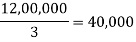 |  |  |
Maximum = 50,000 • decision is A1, using Maximax.
Maximum average is 42,000. • decision is A2,using Laplace criterion.
To find decision under minimax regret, construct the regret table first.
STATES OF NATURE | ACTS (STRATEGIES) | ||
 |  |  | |
 | 10,000 | 0 | 15,000 |
 | 0 | 4,000 | 40,000 |
 | 0 | 0 | 0 |
Maximum | 10,000 | 4,000 | 40,000 |
Minimax = 4,000 which corresponds to .
.
Let us tabulate the decisions using different approaches.
CRITERIA | DECISION |
Optimistic | 
|
Laplace (Equiprobable)
| 
|
Minimax Regret
|  |
The decision depends upon which approach the decision maker wants to consider.
EMV- it is an integral part of risk management. We use it to perform quantitative risk analysis process.
The EMV process involves mathematical calculations. It is a statistical technique in risk management used to quantify risks and calculate the contingency reserve.
EMV = probability 
The EVM will be negative for negative risks and positive for positive risks.
Steps to calculate EMV
1. Assign a probability of occurrence for the risk.
2. Assign monetary value of the impact of the risk when it occurs.
3. Multiply the values produced by step 1 and step 2.
These sums are them added to the project cost to calculate total EMV.
Example: If we have identified risk with a 40% chance of occurring. If this risk occur, it may cost us Rs.6000.
Calculate the EMV
Sol. Here,
The probability of risk is 40%
And impact of risk is (-Rs. 6000)
As we know that-
EMV = probability 
EMV = 0.4
The EMV of the risk event is Rs. -2400
Example: If we have identified an opportunity with a 60% chance of occurring, however it may help us gain Rs. 4000 if this risk occurs.
Calculate EMV.
Sol.
Here we have,
The probability of risk is 60%
And impact of risk is Rs. 4000
As we know that-
EMV = probability 
EMV = 0.6
The EMV of the risk event is Rs. 2400.
Example: Suppose if our team is making a risk management program, and we identify three risks with probabilities of 20%, 30% and 50%. If the first two risks occur, will cost us 7000 rupees and Rs. 8000, however the third will give us Rs. 9000.
Now determine the EMV.
Sol.
We will find EMV one by one-
Here we have,
For first event-
The probability of risk is 20%
And impact of risk is Rs. (-7000)
As we know that-
EMV = probability 
EMV = 0.2
The EMV of the risk event is Rs. -1400.
For second event-
The probability of risk is 30%
And impact of risk is Rs. (-8000)
As we know that-
EMV = probability 
EMV = 0.3
The EMV of the risk event is Rs. -2400.
For third event-
The probability of risk is 50%
And impact of risk is Rs. (9000)
As we know that-
EMV = probability 
EMV = 0.5
The EMV of the risk event is Rs. 4500.
Now we will calculate EMV for all three events-
EMV for all three events = EMV of the first event + EMV of the second event + EMV of the third event

Hence the EMV is 700 for three events.
Key takeaways-
1) EMV- it is an integral part of risk management. We use it to perform quantitative risk analysis process.
EMV = probability 
What is Decision Tree Analysis?
Decision tree analysis is a graphic representation of the various alternative solutions available to solve a problem. When making a choice, the explanation is often decisive. Decision tree analysis is created by answering a few questions that continue until you make the final choice, each time you get a positive or negative answer.
Decision Process
Decision tree analysis is a scientific model and is often used in an organization's decision-making process. When making decisions, management already envisions alternative ideas and solutions. Decision trees provide a graphical representation of alternative solutions and possible choices, which makes it easier to make informed choices. This graphic representation is characterized by a tree-like structure that allows decision-making problems to be viewed in the form of flowcharts, each with a branch of alternative options.
What if
Decision tree analysis makes good use of the "what if" idea. There are several options that take into account both the risks and benefits that a particular choice may pose. The decision tree becomes clear about the outcome of the decisions made, as possible alternatives are also clearly displayed.
Expression
There are several ways to represent a decision tree. This analysis is usually represented by lines, squares, and circles. Squares represent decisions, lines represent results, and circles represent uncertain results. Keeping the lines as far apart gives you plenty of space to add new considerations and ideas.
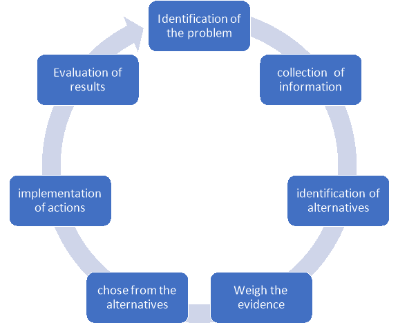
A decision tree representation can be created in four steps:
- Explain the decisions you need to make in the square.
- Draw different lines from the square and write a possible solution for each line.
- Put the result of the solution at the end of the line. Uncertain or uncertain decisions are in a circle. The latter can be placed in a new square when the solution leads to a new decision.
- Each of the squares and circles is critically reviewed for the final choice
Example of Decision Tree Analysis
Suppose a for-profit company wants to increase sales and related profits next year.
You can then use the decision tree to map different alternatives. There are two options for increasing both sales and profits: 1-increasing advertising costs and 2-expanding sales activities. This will create two branches. Option 1 to 2 new options are born. That is, 1-1 is the new agency and 1-2 is to use the services of the existing agency. Option 2 presents two follow-up options in sequence. 2-1-Collaboration with agents or use of 2-2-Original sales support system.
The branch continues.
The next choice from 1-1 is:
1-1-1 Budget will increase by 10%-> Final result: Sales will increase by 6% and profit will increase by 2%
1-1-2 Budget will increase by 5%-> Final result: Sales will increase by 4% and profit will increase by 1.5%
Alternatives resulting from 1.2:
1-2-1 Budget increased by 10%-> Final result: Sales increased by 5%, profit increased by 2.5%
1-2-2 Budget increased by 5%-> Final result: Sales increased by 4%, profit increased by 12%
From 2.1 onwards it will probably look like this:
2-1-1 Setup with own dealer-> Final result: Sales increased by 20%, profit increased by 5%
2-1-2 Cooperation with existing dealers-> Final result: Sales increased by 12.5%, profit increased by 8%
From 2.2 onwards it will probably look like this:
2-2-1 Recruitment of new sales staff-> Final result: Sales increased by 15%, profit increased by 5%
2-2-2 Motivate existing sales staff-> End result: Sales will increase by 4% and profit will increase by 2%.The above example probably shows that the company chooses 1-2-2. This is because the forecast for this decision will increase profits by 12%.
This analysis provides clear proof and is especially useful in situations where it may be desirable to develop various alternatives to decision making in a structured way. This method is increasingly being used by practitioners and technicians to make diagnoses and identify car problems.
Key takeaways:
- Decision theory is an interdisciplinary approach to reaching the most favorable decisions given the uncertain environment.
- Decision theory analyzes the decision-making process by combining psychology, statistics, philosophy, and mathematics.
- Descriptive, normative, and normative are the three main areas of decision theory, each studying different types of decision-making.
- Decision trees are diagrams or charts that help you determine course of action and show statistical probabilities.
- Each branch of the choice tree represents a possible decision, result, or reaction. The farthest branch of the tree represents the end result of a particular decision path.
- Another way to ensure a secure environment is for the manager to create a closed system.
- Multiple events can occur in risky situations. In other words, the manager must first check the likelihood and probability of an event occurring or not occurring.
- People use decision trees in a variety of situations, including complex financial and behavioral decision making for business decisions.
- In the decision tree, each end result is assigned a risk and reward weight or number. When a person uses a decision tree to make a decision, they can look at the final result of each and evaluate the advantages and disadvantages.
- However, using a decision tree to estimate the outcome of a decision can also overwhelm the problem at hand and paralyze the analysis.
EOL is the technique used to make decisions under uncertainty, under the assumptions that the probabilities of each state of nature are known.
Under the EOL criterion, the manager calculate the expected value of the opportunity loss values for each alternatives and then he/she chooses the decision that has the minimum EOL.
Steps to calculate EOL
5. Prepare conditional profit table for each course of action and state of nature.
6. Prepare conditional opportunity loss table.
7. Calculate EOL for each course by multiplying the probability by pop loss.
8. Select course of action for which EOL is minimum.
Ex.1. A consumer product company is examining the introduction of a new product with new packaging or replace the existing product at much higher price (A1) or moderate change in the composition of the existing product with new packaging at a small increase in price (A2) or a small change in the composition of the existing product except the word ‘new’ with the negligible increase in price (A3). The three possible states of nature are S1: decrease in sales. The marketing department has worked out the following payoffs in terms of profits. Which strategy should be considered under (I) Minimax Regret (ii) Optimistic (iii) Equip-probability conditions?
States of Nature | A1 | A2 | A3 |
S1 | 30,000 | 40,000 | 25,000 |
S2 | 50,000 | 45,000 | 10,000 |
S3 | 40,000 | 40,000 | 40,000 |
Ans. Optimistic approach is using Maximax criterion.
Equiprobable is using Laplace criterion.
States of Nature | A1 | A2 | A3 |
S1 | 30,000 | 40,000 | 25,000 |
S2 | 50,000 | 45,000 | 10,000 |
S3 | 40,000 | 40,000 | 40,000 |
Maximum | 50,000 | 46,000 | 40,000 |
Average |  |  |  |
Maximum = 50,000 • decision is A1, using Maximax.
Maximum average is 42,000. • decision is A2,using Laplace criterion.
To find decision under minimax regret, construct the regret table first.
STATES OF NATURE | ACTS (STRATEGIES) | ||
 |  |  | |
 | 10,000 | 0 | 15,000 |
 | 0 | 4,000 | 40,000 |
 | 0 | 0 | 0 |
Maximum | 10,000 | 4,000 | 40,000 |
Minimax = 4,000 which corresponds to .
.
Let us tabulate the decisions using different approaches.
CRITERIA | DECISION |
Optimistic | 
|
Laplace (Equiprobable)
| 
|
Minimax Regret
|  |
The decision depends upon which approach the decision maker wants to consider.
Key takeaways-
1) EOL is the technique used to make decisions under uncertainty, under the assumptions that the probabilities of each state of nature are known.
References-
- Mathematics and Statistics for Business – R. S. Bhardwaj – Excel Books.
- Business Mathematics and Statistics – Subhanjali Chopra – Pearson publication.
- Fundamentals of Business Mathematics and Statistics – ICAI – ICAI.
- Business Mathematics and Statistics – Dr. J K Das, N Das – McGraw Hill Education.
- Mathematical and statistical techniques, Dr. Abhilasha S. Magar & Manohar B. Bhagirath
- IGNOU


