Unit-4
Elementary probability theory
In many real life situations when we are unable to forecast the future with complete certainty. That is, in many decisions, we face the uncertainty. This leads to the study and use of the probability theory.
The first attempt to give quantitative measure of probability was made by Galileo (1564-1642), he was an Italian mathematician.
The first foundation was laid by the two mathematicians Pascal and Fermat due to a gambler's dispute in 1654 which led to the creation of a mathematical theory of sprobability by them. Later, important contributions were made by various researchers including Huyghens, Jacob Bernoulli (1654-1705), Laplace (1749-1827), Abraham De-Moivre (1667-1754), and Markov (1856-1922). Thomas Bayes gave an important technical result known as Bayes’ theorem, published after his death in 1763, using which probabilities can be revised on the basis of some new information.
Random Experiment
An experiment in which we know all the possible outcomes but we can not say that or we can not predict that which of them will occur when we perform the experiment.
Suppose we toss a coin, we know that what are possible outcomes, it would be head or tail, but we do not know which one of these two will occur.
So tossing a coin is a random experiment.
Similarly, ‘Throwing a die’ and ‘Drawing a card from a well shuffled pack of 52 playing cards ‘are the examples of random experiment.
Trial
Performing an experiment is called trial, For example-
(i) Throwing a dice,
(ii) Tossing a coin,
(iii) Picking a playing card.
Note-
1. Die: It is a small cube. Dots (number) are marked on its faces. Plural of the die is dice. On throwing a die, the outcome is the number of dots on its upper face.
2. Cards: A pack of cards consists of four suits i.e. Spades, Hearts, Diamonds and Clubs. Each suit consists of 13 cards, nine cards numbered 2, 3, 4, ..., 10, an Ace, a King, a Queen and a Jack or Knave. Colour of Spades and Clubs is black and that of Hearts and Diamonds is red. Kings, Queens and Jacks are known as face cards.
A probability space is a three-tuple (S, F, P) in which the three components are
- Sample space: A non-empty set S called the sample space, which represents all possible outcomes.
- Event space: A collection F of subsets of S, called the event space.
- Probability function: A function P : FR, that assigns probabilities to the events in F.
Odds in favour of an event and odds against an event: If number of favourable ways = m, number of not favourable events = n
(i) Odds in favour of the event 
(ii) Odds against the event 
Key takeaways-
- Random Experiment- An experiment in which we know all the possible outcomes but we can not say that or we can not predict that which of them will occur when we perform the experiment.
- Performing an experiment is called trial
- A non-empty set S called the sample space, which represents all possible outcomes.
Sample space
Set of all possible outcomes of a random experiment is known as sample space and we denote it by S, and the total number of elements in the sample space is known as size of the sample space and is denoted by n(S).
Discrete sample space- Sample space in which sample points are finite or countably infinite is called discrete sample space.
For example-
- If a die is thrown, then the sample space is
S = {1, 2, 3, 4, 5, 6} and n(S) = 6.
2. If a coin is tossed twice or two coins are tossed simultaneously then the sample space is
S = {HH, HT, TH, TT}
3. If a coin is tossed 4 times or four coins are tossed simultaneously then the sample space is
S = {HHHH, HHHT, HHTH, HTHH, THHH, HHTT, HTHT, HTTH, THHT,
THTH, TTHH, HTTT, THTT, TTHT, TTTH, TTTT} and n(S) = 16.
Note-If a random experiment with x possible outcomes is performed n times, then the total number of elements in the sample is 
Key takeaways-
- Set of all possible outcomes of a random experiment is known as sample space.
- Sample space in which sample points are finite or countably infinite is called discrete sample space.
1. Exhaustive Events or Sample Space: The set of all possible outcomes of a single performance of an experiment is exhaustive events or sample space. Each outcome is called a sample point.
In case of tossing a coin once, S = (H, T) is the sample space. Two outcomes - Head and Tail
- constitute an exhaustive event because no other outcome is possible.
2. Trial and Event: Performing a random experiment is called a trial and outcome is termed as event. Tossing of a coin is a trial and the turning up of head or tail is an event.
3. Equally likely events: Two events are said to be ‘equally likely’, if one of them cannot be expected in preference to the other. For instance, if we draw a card from well-shuffled pack, we may get any card. Then the 52 different cases are equally likely.
4. Independent events: Two events may be independent, when the actual happening of one does not influence in any way the probability of the happening of the other.
5. Mutually Exclusive events: Two events are known as mutually exclusive, when the occurrence of one of them excludes the occurrence of the other. For example, on tossing of a coin, either we get head or tail, but not both.
6. Compound Event: When two or more events occur in composition with each other, the simultaneous occurrence is called a compound event. When a die is thrown, getting a 5 or 6 is a compound event.
7. Favourable Events: The events, which ensure the required happening, are said to be favourable events. For example, in throwing a die, to have the even numbers, 2, 4 and 6 are favourable cases.
Odds in favour of an event and odds against an event-
If the number of favourable cases are ‘m’ and the number or not favourable cases are ‘n’.
Then-
1. Odds in favour of the event = m/n
2. Odds against the event = n/m
Key takeaways-
- The set of all possible outcomes of a single performance of an experiment is exhaustive events or sample space.
- Two events are said to be ‘equally likely’, if one of them cannot be expected in preference to the other.
- Two events are known as mutually exclusive, when the occurrence of one of them excludes the occurrence of the other.
In a random experiment, let S be the sample space.
Let A  S and B
  S be the events, then we say that-
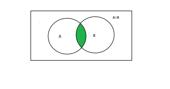
- (A
 B) is an event that occurs only when both A and B occurs.
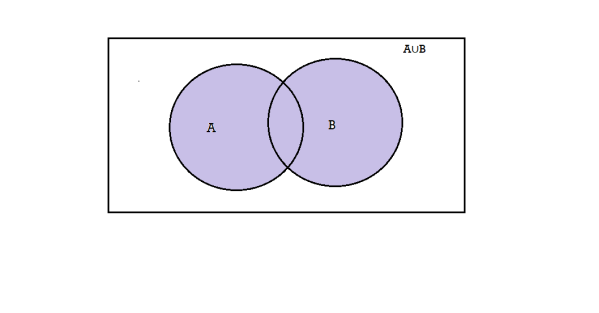
2. (A∪B) is an event that occurs when either one of A or B occurs.
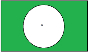
3. A’ is an event that occurs only when A does not occurs.
Let S be the sample space of a random experiment and events A and B  S then
P(A  B) = P(A) + P(B) - P(A
  B)
B)
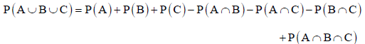
For three non-mutually exclusive events A, B and C, we have
NOTE- If events A and B are mutually exclusive events, then-
P(A  B) = P(A) + P(B)
For three mutually exclusive events A, B and C, we have
P(A  B
B ) = P(A) + P(B) + P(C)
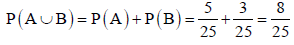
Example: 25 lottery tickets are marked with first 25 numerals. A ticket is drawn at random. Find the probability that it is a multiple of 5 or 7.
Sol.
Let A be the event that the drawn ticket bears a number multiple of 5 and B be the event that it bears a number multiple of 7.
Therefore,
A = {5, 10, 15, 20, 25}
B = {7, 14, 21}
Here, as A 
Therefore, A and B are mutually exclusive, and hence
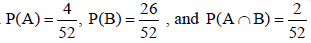
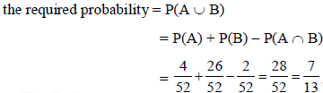
Example: A Card is drawn from a pack of 52 playing cards, find the proabability that the drawn card is an ace or a red colour card.
Sol.
Let A be the event that the drawn card is a card of ace and B be the event that it is red colour card. Now as there are four cards of ace and 26 red colour cards in a pack of 52 playing cards. Also, 2 cards in the pack are ace cards of red colour.
Key takeaways-
- P(A
 B) = P(A) + P(B)
 - P(A
 B
B ) = P(A) + P(B) + P(C)
Exhaustive Cases-
The total number of possible outcomes in a random experiment is called the exhaustive cases.
Or
The number of elements in the sample space is known as number of exhaustive cases
For example:
- When we toss a coin, then the number of exhaustive cases is 2 and the sample space in this case is {H, T}.
- When we throw a die then number of exhaustive cases is 6 and the sample space in this case is {1, 2, 3, 4, 5, 6}
Mutually Exclusive Cases
If the happening of any one of them prevents the happening of all others in a single experiment, then this case is said to be mutually exclusive.
For example:
In throwing a dice experiment all 1, 2, 3, 4, 5, 6 are mutually exclusive as there cannot be simultaneous occurrence 1, 2, 3, 4, 5, 6.
Complementary events
Two events are said to be complementary events when one event occur iff other does not.
The possibility of two complementary events adds up to 1.
The complement of A is denoted by A’
Note- P(A) + P(A’) = 1 Or P(A) = 1 – P(A’)
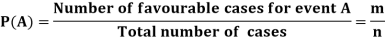
Classical Definition of Probability
Suppose there are ‘n’ exhaustive cases in a random experiment which is equally likely and mutually exclusive.
Let ‘m’ cases are favourable for the happening of an event A, then the probability of happening event A can be defined as-
Probability of non-happening of the event A is defined as-
Note- Always remember that the probability of any events lies between 0 and 1.

Note- Probability of an impossible event is always zero and that of certain event is 1.
The classical definition of probability fails if-
- The cases are not equally likely.
- The number of exhaustive cases is indefinitely large.
Expected value-
Let  are the probabilities of events and
  respectively. Then the expected value can be defined as-

Example1:
In poker, a full house (3 cards of one rank and two of another, e.g. 3 fours and 2 queens) beats a flush (five cards of the same suit).
A player is more likely to be dealt a flush than a full house. We will be able to precisely quantify the meaning of “more likely” here.
Example2:
A coin is tossed repeatedly.
Each toss has two possible outcomes:
Heads (H) or Tails (T)
Both equally likely. The outcome of each toss is unpredictable; so is the sequence of H and T.
However, as the number of tosses gets large, we expect that the number of H (heads) recorded will fluctuate around of the total number of tosses. We say the probability of a H is
  , abbreviated by
 . Of course
  also
also
NOTES:
• In general, an event has associated to it a probability, which is a real number between 0 and 1.
• Events which are unlikely have low (close to 0) probability, and events which are likely have high (close to 1) probability.
• The probability of an event which is certain to occur is 1; the probability of an impossible event is 0.
Example: A bag contains 7 red and 8 black balls then find the probability of getting a red ball.
Sol.
Here total cases = 7 + 8 = 15
According to the definition of probability,
So that, here favourable cases- red balls = 7
Then,

Example: A bag contains 4 red, 5 black and 2 green balls. One ball is drawn from the bag. Find the probability that-
(i) It is a red ball
(ii) It is not black
(iii) It is green or black
Sol.
There are total 11 exhaustive cases.
- We know that, by the definition

And the favourable cases are 4, then the probability of getting a red ball is-

Similarly-
Probability of getting a ball which is not black is-

Probability of getting a green or black ball is-

Example: A fair die is thrown. Find the probability of getting
(i) A prime number.
(ii) An even number.
(iii) A number multiple of 2 or 3.
(iv) A number multiple of 2 and 3.
(v) A number greater than 4.
Sol:
The sample space in this case is- S = {1, 2, 3, 4, 5, 6}
(i) Let E1 be the event of getting a prime number, then E1 = {2, 3, 5}.
P(E1) = 3/6 or ½
(ii) Let E2 be the event of getting an even number, then
E2 = {2, 4, 6}.
P(E2) = 3/6 or ½
(iii) Let E3 be the event of getting an even number, then
E3 = {2, 3, 4, 6 }
P(E3) = 4/6 or 2/3
(iv) Let E4 be the event of getting an even number, then
E4 = {6}.
P(E4) = 1/6
(v) Let E5 be the event of getting an even number, then
E4 = {5, 6}.
P(E5) = 2/6 = 1/3
Key takeaways-
- Probability of non-happening of the event A is defined as-

2. Always remember that the probability of any events lies between 0 and 1.
Addition and multiplication law of probability-
Addition law-
If  are the probabilities of mutually exclusive events, then the probability P, that any of these events will happen is given by
Note-
If two events A and B are not mutually exclusive then the probability of the event that either A or B or both will happen is given by-

Example: A box contains 4 white and 2 black balls and a second box contains three balls of each colour. Now a bag is selected at random and a ball is drawn randomly from the chosen box. Then what will be the probability that the ball is white?
Sol.
Here we have two mutually exclusive cases-
1. The first bag is chosen
2. The second bag is chosen
The chance of choosing the first bag is 1/2. And if this bag is chosen then the probability of drawing a white ball is 4/6.
So that the probability of drawing a white ball from the first bag is-

And the probability of drawing a white ball from the second bag is-

Here the events are mutually exclusive, then the required probability is-

Example-25 lottery tickets are marked with the first 25 numerals. A ticket is drawn at random.
Find the probability that it is a multiple of 5 or 7.
Sol:
Let A be the event that the drawn ticket bears a number multiple of 5 and B be the event that it bears a number multiple of 7.
So that
A = {5, 10, 15, 20, 25}
B = {7, 14, 21}
Here, as A  B =
B =  ,
,
A and B are mutually exclusive
Then,
Multiplication law-
For two events A and B-

Here  is called conditional probability of B given that A has already happened.
Now-
If A and B are two independent events, then-
Because in the case of independent events- 
Example: A bag contains 9 balls, two of which are red three blue, and four black.
Three balls are drawn randomly. What is the probability that-
1. The three balls are of different colours.
2. The three balls are of the same colours.
Sol.
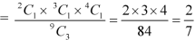
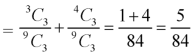
1. Three balls will be of a different colour if one ball is red, one blue and one black ball are drawn-
Then the probability will be-
2. Three balls will be of the same colour if one ball is red, one blue and one black ball are drawn-
Then the probability will be-
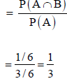
Example: A die is rolled. If the outcome is a number greater than three. What is the probability that it is a prime number?
Sol.
The sample space is- S = {1, 2, 3, 4, 5, 6}
Let A be the event that an outcome is a number that is greater than three and B be the event that it is a prime.
So that-
A = {4, 5, 6} and B = {2, 3, 5} and hence 
P(A) = 3/6, P(B) = 3/6 and 
Now the required probability-
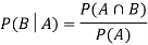


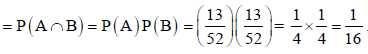
Example: Two cards are drawn from a pack of playing cards in succession with the replacement of the first card. Find the probability that both are the cards of heart.
Sol.
Let A be the event that the first card drawn is a heart and B be the event that the second card is a heart card.
As the cards are drawn with replacement,
Here A and B are independent and the required probability will be-
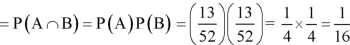
Example: Two male and female candidates appear in an interview for two positions in the same post. The probability that the male candidate is selected is 1/7 and the female candidate selected is 1/5.
What is the probability that-
1. Both of them will be selected
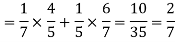
2. Only one of them will be selected
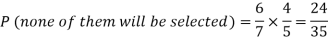
3. None of them will be selected.
Sol.
Here, P (male’s selection) = 1/7
And
P (female’s selection) = 1/5
Then-
1.
2.

3.
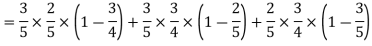
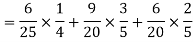
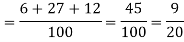
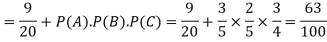
Example: A can hit a target 3 times in 5 shots, B 2 times in 5 shots, and C 3 times in 4 shots. All of them fire one shot each simultaneously at the target.
What is the probability that-
1. Two shots hit
2. At least two shots hit
Sol.
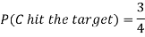
1. Now probability that 2 shots hit the target-

2.
Probability of at least two shots hitting the target

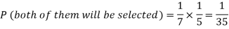
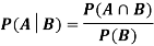
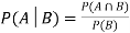
Let A and B be two events of a sample space Sand let  . Then conditional probability of the event A, given B, denoted by
 is defined by –
Theorem: If the events Aand Bdefined on a sample space S of a random experiment are independent, then

Example1: A factory has two machines A and B making 60% and 40% respectively of the total production. Machine A produces 3% defective items, and B produces 5% defective items. Find the probability that a given defective part came from A.
SOLUTION:
We consider the following events:
A: Selected item comes from A.
B: Selected item comes from B.
D: Selected item is defective.
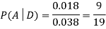
We are looking for  . We know:

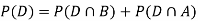
Now,
So we need


Since, D is the union of the mutually exclusive events  and
and  (the entire sample space is the union of the mutually exclusive events A and B)


Example2: Two fair dice are rolled, 1 red and 1 blue. The Sample Space is
S = {(1, 1),(1, 2), . . . ,(1, 6), . . . ,(6, 6)}.Total -36 outcomes, all equally likely (here (2, 3) denotes the outcome where the red die show 2 and the blue one shows 3).
(a) Consider the following events:
A: Red die shows 6.
B: Blue die shows 6.
Find ,
,  and
and  .
.
Solution:
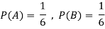

NOTE:
 so
so 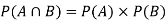 for this example. This is not surprising - we expect A to occur in
  of cases. In
  of these cases i.e. in
  of all cases, we expect B to also occur.
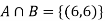
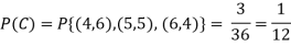
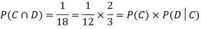
(b) Consider the following events:
C: Total Score is 10.
D: Red die shows an even number.
Find  ,
,  and
and  .
.
Solution:

NOTE:
 so,
so,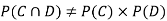 .
.
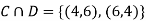
Why does multiplication not apply here as in part (a)?
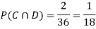
ANSWER: Suppose C occurs: so the outcome is either (4, 6), (5, 5) or (6, 4). In two of these cases, namely (4, 6) and (6, 4), the event D also occurs. Thus
Although , the probability that D occurs given that C occurs is
  .
.
We write , and call
  the conditional probability of D given C.
NOTE: In the above example
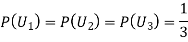
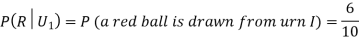
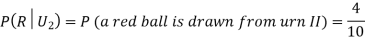
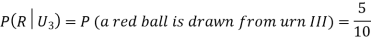
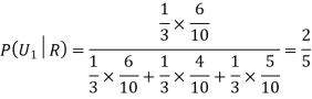
Example3: Three urns contain 6 red, 4 black; 4 red, 6 black; 5 red, 5 black balls respectively. One of the urns is selected at random and a ball is drawn from it. If the ball drawn is red find the probability that it is drawn from the first urn.
Solution:
 :The ball is drawn from urnI.
 : The ball is drawn from urnII.
 : The ball is drawn from urnIII.
R:The ball is red.
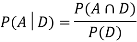
We have to find 

Since the three urns are equally likely to be selected
Also,
From (i), we have
Key takeaways-

Independence of events:
Events are said to be independent if happening or non-happening of any one event is not affected by the happening or non-happening of other events. For example, if a coin is tossed certain number of times, then happening of head in any trial is not affected by any other trial i.e. all the trials are independent.
Two events A and B are independent if and only if P(B|A) = P(B) i.e. there is no relevance of giving any information. Here, if A has already happened, even then it does not alter the probability of B.
If A and B are independent events then-
(Two disjoint events are not independent.)
Independence implies that

Knowing that outcome is in B does not change your perception of the outcome’s being in A.
Note-
- Mutually exclusive events can never be independent.
- If events A and B are independent then-
- A and B’ are independent.
- A’ and B are independent.
- A’ and B’ are independent.
Example: Two cards are drawn from a pack of cards in succession with replacement of first card. Find the probability that both are the cards of ‘heart’.
Sol.
Let A be the event that the first card drawn is a heart card and B be the event that second card is a heart card.
As the cards are drawn with replacement,
Here A and B are independent and hence the required probability
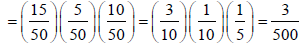
Example: A class consists of 10 boys and 40 girls. 5 of the students are rich and 15 students are brilliant. Find the probability of selecting a brilliant rich boy.
Sol.
Let A be the event that the selected student is brilliant, B be the event that he/she is rich and C be the event that the student is boy.
P(A) = 15/50, P(B) = 5/50 and P(C) = 10/50,
Hence the required probability- [ A, B, C are independent events]

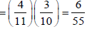
Example: An urn contains 4 red and 7 blue balls. Two balls are drawn one by one without replacement. Find the probability of getting 2 red balls.
Sol:
Let A be the event that first ball drawn is red and B be the event that the second ball drawn is red.
P(A) = 4 /11 and P(B|A) = 3/10
The required probability = P(A and B)
= P(A) P(B|A)
Example: A die is rolled. If the outcome is a number greater than 3, what is the probability that it is a prime number?
Sol:
The sample space of the experiment is
S = {1, 2, 3, 4, 5, 6}
Let A be event that the outcome is a number greater than 3 and B be the event that it is a prime number.
A = {4, 5, 6}, B = {2, 3, 5} and hence
P(A) = 3/6, P(B) = 3/6,  1/6.
1/6.
The required probability = P(B|A)
Key takeaways-
- Two events A and B are independent if and only if P(B|A) = P(B)
- If A and B are independent events then-
3. Mutually exclusive events can never be independent.
A random variable is said to be discrete if it has either a finite or a countable number of values
The number of students present each day in a class during an academic session is an example of discrete random variable as the number cannot take a fractional value.
Probability mass function-
Let X be a r.v. Which takes the values  and let P[X =
  ] = p(
 . This function p(xi), i =1,2, … defined for the values
  assumed by X is called probability mass function of X satisfying p(xi) ≥ 0 and
Example: A random variable x has the following probability distribution-
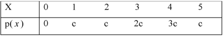
Then find-
1. Value of c.
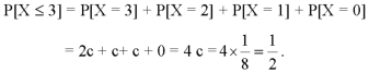
2. P[X≤3]
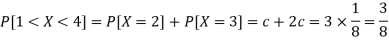
3. P[1 < X <4]
Sol.
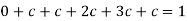
We know that for the given probability distribution-

So that-


2.
3.
Example: Find the probability distribution of the number of heads when three fair coins are tossed simultaneously.
Sol:
Let X be the number of heads in the toss of three fair coins.
As the random variable, “the number of heads” in a toss of three coins may be
0 or 1 or 2 or 3 associated with the sample space
{HHH, HHT, HTH, THH, HTT, THT, TTH, TTT},
X can take the values 0, 1, 2, 3, with
P[X = 0] = P[TTT ] = 1/8
P[X = 1] = P[HTT, THT, TTH] = 3/8
P[X = 2] = P[HHT, HTH, THH] = 3/8
P[X = 3] = P [HHH] = 1/8
Probability distribution of X, i.e. the number of heads when three coins are tossed simultaneously is
X | 0 | 1 | 2 | 3 |
p(x) | 1/8 | 3/8 | 3/8 | 1/8 |
Independent random variables-
Two discrete random variables X and Y are said to be independent only if-

Note- Two events are independent only if 
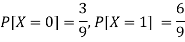
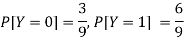
Example: Two discrete random variables X and Y have-

And
P[X = 1, Y = 1] = 5/9.
Check whether X and Y are independent or not?
Sol.
First we write the given distribution In tabular form-
X/Y | 0 | 1 | P(x) |
0 | 2/9 | 1/9 | 3/9 |
1 | 1/9 | 5/9 | 6/9 |
P(y) | 3/9 | 6/9 | 1 |
Now-
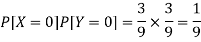
But
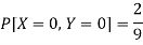
So that-

Hence X and Y are not independent.
Infinite sequence of Bernoulli trials
Let a product is tested which may be defective or non-defective, let p be the probability of non-defective and q = 1 - p be the probability of defective product.
And let X be a random variable which takes 1 if success occurs and 0 if failure occurs.
Therefore-
P[X = 1] = p
P[X = 0] = q = 1- p
This experiment is known as a Bernoulli trial and the random variable X is a Bernoulli variable.
Conditions for Bernoulli tests
1. A finite number of tests.
2. Each trial must have exactly two results: success or failure.
3. The tests must be independent.
4. The probability of success or failure must be the same in each test.
Bernoulli distribution-
A discrete random variable said to be follow a Bernoulli distribution with parameter p if its p.m.f is given by-

Bernoulli distribution in tabular form can be given as-
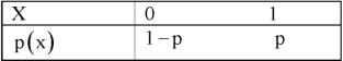
1. Mean of the Bernoulli distribution is p.
2. Variance = p(1-p)
Example: If X be a random variable following a Bernoulli distribution with parameter p = 0.6, then find its mean and variance.
Sol.
Mean = p = 0.6
Variance = p(1-p) = 0.6 (1 – 0.6) = 0.6 ×0.4 = 0.24
Example: If the probability that a light bulb is defective is 0.8, what is the probability that the light bulb is not defective?
Solution:
Probability that the bulb is defective, p = 0.8
Probability that the bulb is not defective, q = 1 - p = 1 - 0.8 = 0.2
Example: 10 coins are tossed simultaneously where the probability of getting heads for each coin is 0.6. Find the probability of obtaining 4 heads.
Solution:
Probability of obtaining the head, p = 0.6
Probability of obtaining the head, q = 1 - p = 1 - 0.6 = 0.4
Probability of obtaining 4 of 10 heads, P (X = 4) = C104 (0.6) 4 (0.4) 6P (X = 4) = C410 (0.6) 4 (0.4) 6 = 0.111476736
Example: In an exam, 10 multiple-choice questions are asked where only one in four answers is correct. Find the probability of getting 5 out of 10 correct questions on an answer sheet.
Solution:
Probability of obtaining a correct answer, p = 1414 = 0.25
Probability of obtaining a correct answer, q = 1 - p = 1 - 0.25 = 0.75
Probability of obtaining 5 correct answers, P (X = 5) = C105 (0.25) 5 (0.75) 5C510 (0.25) 5 (0.75) 5 = 0.05839920044
Binomial distribution-
This distribution was discovered by a Swiss mathematician Jame Bernoulli (1654-1705) and is also known as Bernoulli Distribution.
The conditions for binomial distribution-
- The number of trials is finite and fixed.
- In every trial there are only two possible outcomes success or failure.
- The trials are independent. The outcome of one trial does not affect the other trial.
- p, the probability of success from trial to trial is fixed and q the probability of failure is equal to 1-p. This is the same in all the trials.
Definition-
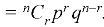
A discrete random variable X is said to be follow the binomial distribution with parameter n and p.
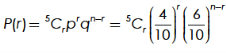
The probability of happening of an event r times exactly in n trials is-
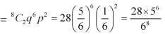
Example: A die is thrown 8 times then find the probability that 3 will show-
1. Exactly 2 times
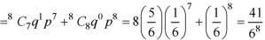
2. At least 7 times
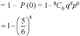
3. At least once
Sol.
As we know that-
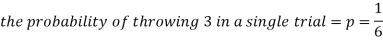
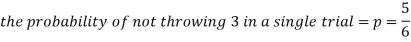
Then-
1. Probability of getting 3 exactly 2 times will be-
2. Probability of getting 3 at least 7 or 8 times will be-
3. Probability of getting 3 at least once or (1 or 2 or 3 or 4 or 5 or 6 or 7 or 8 times)-

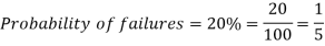
Example: If the percentage of failure in a test is 20. If six students appear in the test, then what will be the probability that at least five students will pass the test?
Sol.
Here
Then the probability of at least five students will pass the test-
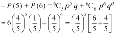
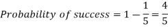
Example: The probability that an evening college student will graduate is 0.4. Determine the probability that out of 5 students (a) none, (b) one, and (c) atleast one will graduate.
Sol.
Here
n = 5, p = 0.4 or 4/10, q = 0.6 = (6/10)
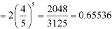
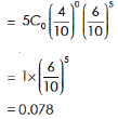
a) The probability of zero success-
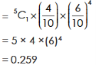
(b) The probability of one success-
(c) The probability of atleast one success
= 1– probability of no success
= 1– 0.078
= 0.922
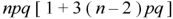
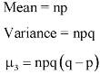
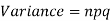
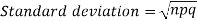
Mean and standard deviation of binomial distribution-
1. 
2. 
3. 
Moments of binomial distribution-
1. First moment about the origin-
2. Second moment about the origin-
3. Third moment about origin-

4. Fourth moment about origin-

5. Third central moment-

6. Fourth central moment-
Example: Find mean and variance of a binomial distribution with p = 1/4 and n = 10.
Sol.
Here 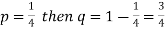
Mean = np = 
Variance = npq = 
Example: If a dice is rolled thrice. A success is getting 1 or 6 on a roll. Find the mean variance of the number of success.
Sol.
Here n = 3 , p = 1/3 and q = 2/3
Mean = np = 1
And variance = npq = 2/3
5.1.2. Poisson distribution
Poisson distribution-
Poisson distribution was derived in 1837 by a French mathematician Simeon D Poisson (1731-1840).
Examples of Poisson distribution-
- The number of defective articles produced by a quality machine,
- The number of persons dying due to rare disease or snake bite etc.
- The number of accidental deaths by falling from trees or roofs etc.
- The number of cars passes on road within a fixed period.
Poisson distribution is a limiting case of binomial distribution under certain conditions listed below-
1. n, the number of trials are infinitely large.
2. p, the probability of success for each trial is very small.
3. Np is finite quantity say 
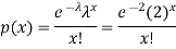
A random variable X is said to be follow Poisson distribution if it has the following probability mass function-
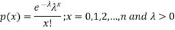
Moments of Poisson distribution-
1. First moment about origin-  which Is known as mean.
2. Second moment about origin- 
3. Third moment about origin- 
4. Fourth moment about origin- 
Note-
1. Poisson distribution is always positively skewed distribution.
2. Mean and variance of Poisson dist. Are always equal
For Poisson distribution-

Example: If cars arriving at workshop follow the Poisson distribution. If the average number of cars arrivals during a specified period of an hour is 2.
Find the probabilities that during the given hour-
1. No car arrive
2. At least two cars arrive.
Sol.
Here the average of car arrivals is - 2
So that mean = 2

Let X be the number of cars arriving during the given hour,
By using Poisson distribution, we get-
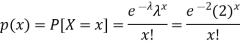
So that the required probability-
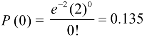
1. P [no car will arrive] = P [X = x] = 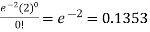
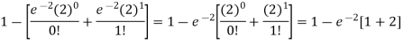
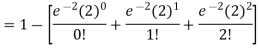
2. P [At least two cars will arrive] = P [X≥2] = P [X =2] + P [X = 3] + ……….
= 1 - P [[X =1] + P [X =0]]

Example: If the probability that a vaccine given to the patients shows bad reaction is 0.001, then find the probability that out of 2000 patients-
1. Exactly 3 patients
2. More than 2 patients
3. No patient
Will show bad reaction.
Sol.
Here p = 0.001 and number of patients (n) = 2000
Then 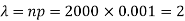
By using Poisson distribution, we get-
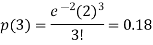
1. Probability that exactly 3 patients show bad reaction is-
2. Probability that more than 2 patients show bad reaction-


3. Probability that no patient shows bad reaction-
Example: If a book has 600 pages and it has 40 printing mistakes. Assume that these mistakes are randomly distributed and x the number of mistakes per page follow Poisson distribution.
What is the probability that there will not be any mistake if 10 pages selected at random?
Sol.
Here 
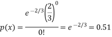
We get by using Poisson distribytion-
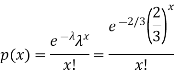
Then-
Key takeaways-
- A random variable is said to be discrete if it has either a finite or a countable number of values
- The probability of happening of an event r times exactly in n trials is-

3. Mean and standard deviation of binomial distribution-

4. Poisson dist- 

5. Poisson distribution is always positively skewed distribution.
6. Mean and variance of Poisson dist. Are always equal
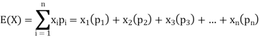
Expectations of discrete random variables
Let a random variable X has a probability distribution which assumes the values say with their associated probabilities
  then the mathematical expectation can be defined as-
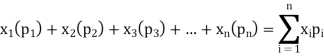
The expected value of a random variable X is written as E(X).
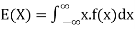
Expected value for a continuous random variable is
Properties of expectation:
- E(k) = k, where k is a constant
- E(kX) = kE(X), k being a constant.
- E(aX + b) = aE(X) + b, where a and b are constants
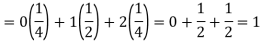
Example: If a random variable X has the following probability distribution in tabular form then what will be the expected value of X.
X | 0 | 1 | 2 |
P(x) | 1/4 | 1/2 | 1/4 |
Sol.
We know that-
So that-
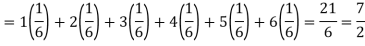
Example: Find the expectations of the number of an unbiased die when thrown.
Sol. Let X be a random variable which represents the number on a die when thrown.
X can take the values-
1, 2, 3, 4, 5, 6
With
P[X = 1] = P[X = 2] = P[X = 3] = P[X = 4] = P[X = 5] = P[X = 6] = 1/6
The distribution table will be-
X | 1 | 2 | 3 | 4 | 5 | 6 |
p(x) | 1/6 | 1/6 | 1/6 | 1/6 | 1/6 | 1/6 |
Hence the expectation of number on the die thrown is-

So that-
Example: If it rains, a rain coat dealer can earn Rs 500 per day. If it is a dry day, he can lose Rs 100 per day. What is his expectation, if the probability of rain is 0.4?
Sol.
Let X be the amount earned on a day by the dealer. Therefore, X can take the values Rs 500, -Rs 100
Loss of 100 Rs is equivalent to -100 Rs
| Rainy day | Dry day |
X(in Rs) | 500 | -100 |
p(x) | 0.4 | 0.6 |
Hence the expectation of the amount earned-
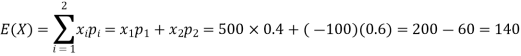
Thus, his expectation is Rs 140, i.e. on an overage he earns Rs 140 per day.
Variance
Variance of a random variable X is defined as the second order central moment and it is defined as-
Or

Note-
If X is a random variable, then-

Where a and b are constants.
Note-

Example: Find the following of the given probability distribution-
X | -2 | -1 | 0 | 1 | 2 |
p(x) | 0.15 | 0.30 | 0 | 0.30 | 0.25 |
- V(X)
- V (2X + 3)
Sol.
- We know that-

2. V(2X + C) = 
Key takwaways-


References-
- Mathematics and Statistics for Business – R. S. Bhardwaj – Excel Books.
- Business Mathematics and Statistics – Subhanjali Chopra – Pearson publication.
- Fundamentals of Business Mathematics and Statistics – ICAI – ICAI.
- Business Mathematics and Statistics – Dr. J K Das, N Das – McGraw Hill Education.
- Mathematical and statistical techniques, Dr. Abhilasha S. Magar & Manohar B. Bhagirath
- IGNOU


