UNIT-4
Adaptive Filter
Adaptive signal processing has many points of similarity to adaptive control. There are, however, many important differences in emphasis leading to differences in the algorithms and in the analysis. The following points were discussed at the round table:
1.In adaptive control we have measurements of both the input and the output of the plant. In adaptive processing the “plant” is a signal model whose input is unknown.
2.In control application the plant is often stable and minimum phase. The models encountered in signal processing have poles near or on the unit circle and are often non-minimum phase.
3.In adaptive filters it is often necessary to impose various constraints on the filter parameters (linear phase characteristics, equiripple pass-band, etc.). These constraints complicate the derivation and analysis of the adaptive algorithm.
4.In signal processing problem the measurements are often extremely noisy. In control problems the measurement system is usually designed to provide relatively noise-free information.
5.It analyzes the information and manipulates the signal on each source. Time-frequency modeling and spectral masking operation are implemented in a way of front-end signal processing. Source localization is identified by using a microphone array. Through signal processing, we judge how the sources are mixed. The input signals are processed to obtain the separated signals through several processing components. Therefore, front-end processing includes the frequency-domain audio source separation which could align the permutation and magnitude ambiguities, separate the convolutive mixtures, identify the number of sources, resolve the overdetermined/underdetermined problem, and compensate for the room reverberation.
An FIR system has a finite-duration impulse response that is zero outside of some finite time interval. Thus, an FIR system has a finite memory of length-N samples. Three basic structures for realizing the FIR filter (transversal, symmetric, and lattice) are described below.
Transversal Structure
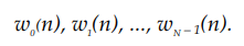
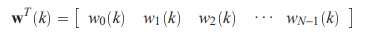
The figure below shows the structure of a transversal FIR filter with N tap weights (adjustable during the adaptation process) with values at time n denoted as
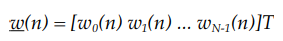
The tap-weight vector, w(n), is represented as
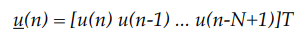
the tap-input vector, u(n), as
The FIR filter output, y(n), can then be expressed as
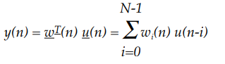
where T denotes transpose, n is the time index, and N is the order of the filter.
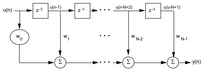
Fig.1: Transversal Structure
Symmetric Transversal Structure
The characteristic of linear phase response in a filter is sometimes desirable because it allows a system to reject or shape energy bands of the spectrum and still maintain the basic pulse integrity with a constant filter group delay. Imaging and digital communications are examples of applications where this characteristic is desirable. An FIR filter with time domain symmetry, such as
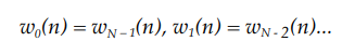
has a linear phase response in the frequency domain. Consequently, the number of weights is reduced by a half in a transversal structure, as shown in Figure with an even N tap weights. The tap-input vector becomes

As a result, the filter output y(n) becomes
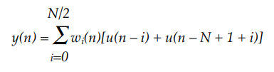
Fig.2: Symmetric Transversal Structure
Lattice Structure
The lattice filter has a modular structure with cascaded identical stages. Figure shows one stage of a lattice FIR structure.
The lattice structure offers several advantages over the transversal structure:
• The lattice structure has good numerical round-off characteristics that make it less sensitive than the transversal structure to round-off errors and parameter variations.
• The lattice structure orthogonalizes the input signal stage-by-stage, which leads to fast convergence and efficient tracking capabilities when used in an adaptive environment.
• The various stages are decoupled from each other, so it is relatively easy to increase the prediction order if required.
• The lattice filter (predictor) can be interpreted as wave propagation in a stratified medium. This can represent an acoustical tube model of the human vocal tract, which is extremely useful in digital speech processing.
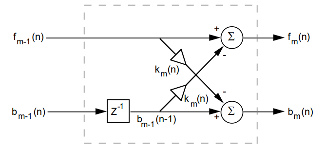
Fig.3: Lattice structure
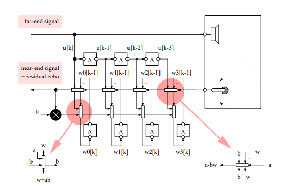
Fig. LMS algorithm
Many of the adaptation schemes we will encounter take the form
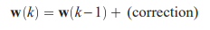
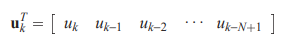
where
contains the tap weights at time k. We have already indicated that the error signal often used to steer the adaptation, and so one has
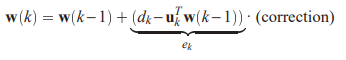
where
This make sense since if the error is small then we do not need to alter the weight; on the other hand, if the error is large, we will need a large change in the weights. Note that the correction term has to be a vector – W(k) is one! Its role is specify the ‘direction’ in which one should move in going from w(k-1) to w(k). Different schemes have different choices for the correction vector. A simple scheme, known as the Least Mean Squares (LMS) algorithm (Widrow 1965), uses the FIR filter input vector as a correction vector, i.e.
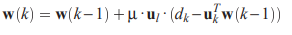
where µ is a so-called step size parameter, that controls the speed of the adaptation. Proper tuning of the µ will turn out to be crucial to obtain stable operation. The LMS algorithm is seen to be particularly simple to understand and implement, which explains why it is used in so many applications. The class of algorithms so derived, is referred to as the class of Recursive Least Squares (RLS) algorithms. Typical of these algorithms is an adaptation formula that differs from the LMS formula in that a ‘better’ correction vector is used, i.e.
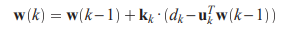
where kk is the so-called Kalman gain vector, which is computed from the autocorrelation matrix of the filter input signal.
References:
1. John G Prokis , “Digital Signal Processing ,Principles, Algorithms and
Application”,PHI
2. S.K.Mitra, “Digital Signal Processing”, TMH
3. E. C. Ifleachor and B. W. Jervis, “Digital Signal Processing- A Practical
Approach”, Second Edition, Pearson education.
4.Avtar Singh, S. Srinivasan, “Digital Signal Processing Implementation using DSP,
Microprocessors with examples from TMS 320C6XXX”, Thomas Publication.


