UNIT 3
IIR Filter Design
The Impulse Invariance Method is used to design a discrete filter that yields a similar frequency response to that of an analog filter. Discrete filters are amazing for two very significant reasons:
We can design this filter by finding out one very important piece of information i.e., the impulse response of the analog filter. By sampling the response we will get the time-domain impulse response of the discrete filter.
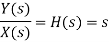
When observing the impulse responses of the continuous and discrete responses, it is hard to miss that they correspond with each other. The analog filter can be represented by a transfer function, Hc(s).
Zeros are the roots of the numerator and poles are the roots of the denominator.
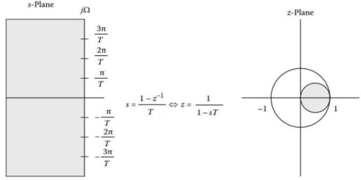
Mapping from s-plane to z-plane
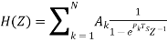
The transfer function of the analog filter in terms of partial fraction expansion with real coefficients is
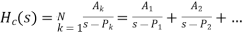 Where A are the real coefficients and P are the poles of the function And k can be 1, 2 …N.
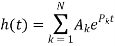
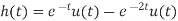
h(t) is the impulse response of the same analog filter but in the time domain. Since ‘s’ represents a Laplace function Hc(s) can be converted to h(t), by taking its inverse Laplace transform.
Using this transformation,
We obtain
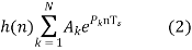
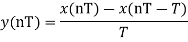
However, in order to obtain a discrete frequency response, we need to sample this equation. Replace ‘nTS’ in the place of t where TS represents the sampling time. This gives us the sampled response h(n),
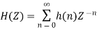
Now, to obtain the transfer function of the IIR Digital Filter which is of the ‘z’ operator, we have to perform z-transform with the newly found sampled impulse response, h(n). For a causal system which depends on past(-n) and current inputs (n), we can get H(z) with the formula shown below
We have already obtained the equation for h(n). Hence, substitute eqn (2) into the above equation
Factoring the coefficient and the common power of n
—(3)
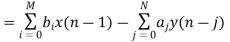
Based on the standard summation formula, (3) is modified and written as the required transfer function of the IIR filter.
 –(4)
–(4)
Hence (4) is obtained from (1), by mapping the poles of the analog filter to that of the digital filter.
That is how you map from the s-plane to z-plane
Relationship of S-plane to Z plane
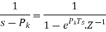
From the equation above, Since, the poles are the denominators we can say  .
.
Comparing (1) and (4), we can derive that
 –(5)
–(5)
and since  , substituting into (5) gives us
 –(6)
–(6)
where
TS is the sampling time
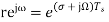
Now, s is taken to be the Laplace operator
 –(7)
–(7)
σ is the attenuation factor
Ω is the analog frequency
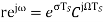
Changing Z from rectangular coordinates to the polar coordinates, we get:
 –(8)
–(8)
where r is magnitude and ω is digital frequency
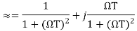
Replacing (7) in place of s in (6), and replacing that value as Z in (8)
Compare the real and imaginary parts separately. Where the component with ‘j’ is imaginary.
 –(9)
–(9)
and

Hence, we can make the inference that

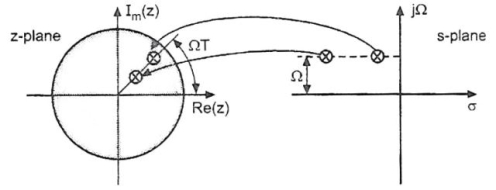
To understand the relationship between the s-plane and Z-plane, we need to picture how they will be plotted on a graph. If we were to plot (7) in the ‘s’ domain, σ would be the X-coordinates and jΩ would be the Y-coordinate. Now, if we were to plot (8) in the ‘Z’ domain, the real portion would be the X-coordinate, and the imaginary part would be the Y-coordinate.
Let us take a closer look at equation (9),

There are a few conditions that could help us identify where it is going to be mapped on the s-plane.
Case 1
when σ <0, it would translate that r is the reciprocal of ‘e’ raised to a constant. This will limit the range of r from 0 to 1.
Since σ <0, it would be a negative value and would be mapped on the left-hand side of the graph in the ‘s’ domain
Since 0<r<1, this would fall within the unit circle which has a radius of in the ‘z’ domain.
Case 2
When σ =0, this would make r=e0, which gives us 1, which means r=1. When the radius is 1, it is a unit circle.
Since σ =0, which indicates the Y-axis of the ‘s’ domain.
Since r=1, the point would be on the unit circle in the ‘z’ domain.
Case 3
When σ>0, since it is positive, r would be equal to ‘e’ raised to a particular constant, which means r would also be a positive value greater than 1.
Since σ>0, the positive value would be mapped onto the right-hand side of the ‘s’ domain.
Since r>1, the point would be mapped outside the unit circle in the ‘z’ domain.
Here is a pictorial representation of the three cases:
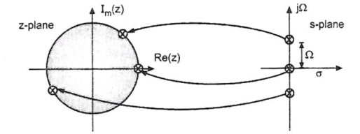
Mapping of poles located at the imaginary axis of the s-plane onto the unit circle of the z-plane. This is an important condition for accurate transformation.
Mapping of the stable poles on the left-hand side of the imaginary s-plane axis into the unit circle on the z-plane. Poles on the right-hand side of the imaginary axis of the s-plane lie outside the unit circle of the z-plane when mapped.
Disadvantages:
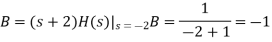
Given 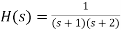 , that has a sampling frequency of 5Hz. Find the transfer function of the IIR digital filter.
Solution:
Step 1:
Step 2:
Applying partial fractions on H(s),

Step 3:

Step 4:
The bilinear transform is the result of a numerical integration of the analog transfer function into the digital domain. We can define the bilinear transform as:

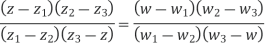
Find the bilinear transformation which maps points z =2,1,0 onto the points w=1,0,i.
Ans. Let, 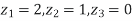
And, 
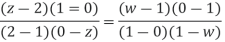
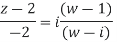
Since bilinear transformation preserves cross ratios,
Thus we have,


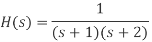
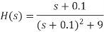
Use the bilinear transformation to convert the analog filtrt with system function

 into a digital IIR filter. Select T =0.1
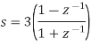
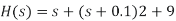
Consider the following system function

Note that the following is the resonant frequency of the analog filter

Consider that the resonant frequency of analog filter must be mapped by selecting the value of parameter
T= 0,1
Use the following mapping for bilinear transformation
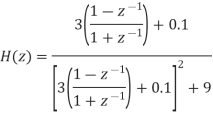
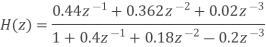
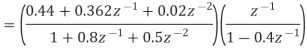
Write the system function H(z) of the resultant digital filter
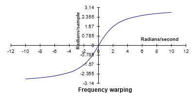
Frequency warping
• The bilinear transformation method has the following important features: A stable analog filter gives a stable digital filter. The maxima and minima of the amplitude response in the analog filter are preserved in the digital filter. As a consequence, – the pass band ripple, and – the minimum stop band attenuation of the analog filter are preserved in the digital filter frame.
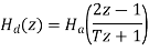
• To determine the frequency response of a continuous-time filter, the transfer function Ha(s)Ha(s) is evaluated at s=jω which is on the jω axis. Likewise, to determine the frequency response of a discrete-time filter, the transfer function Hd(z) is evaluated at z=ejωT which is on the unit circle, |z|=1|z|=1 .
• When the actual frequency of ω is input to the discrete-time filter designed by use of the bilinear transform, it is desired to know at what frequency, ωa , for the continuous-time filter that this ω is mapped to.
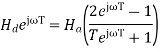
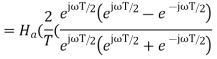
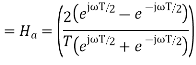
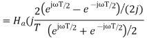
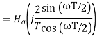
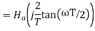
• This shows that every point on the unit circle in the discrete-time filter z-plane, z= ejωT is mapped to a point on the jω axis on the continuous-time filter s-plane, s=jω. That is, the discrete-time to continuous-time frequency mapping of the bilinear transform is
ωa=(2/T) tan(ωt/2)
and the inverse mapping is
ω=(2/T) arc tan(ωaT/2)
• The discrete-time filter behaves at frequency the same way that the continuous-time filter behaves at frequency (2/T)tan(ωT/2). Specifically, the gain and phase shift that the discrete-time filter has at frequency ω is the same gain and phase shift that the continuous-time filter has at frequency (2/T)tan(ωT/2). This means that every feature, every "bump" that is visible in the frequency response of the continuous-time filter is also visible in the discrete-time filter, but at a different frequency. For low frequencies (that is, when ω≪2/T or ωa≪2/T),ω≈ωa.
One can see that the entire continuous frequency range
−∞<ωa<+∞
is mapped onto the fundamental frequency interval
−πT<ω<+πTω=±π/T.ωa=±∞
One can also see that there is a nonlinear relationship between ωa and ω This effect of the bilinear transform is called frequency warping.

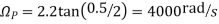
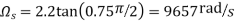
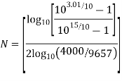
Design a discrete time lowpass filter to satisfy the following amplitude specifications: 

Assume 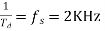
The pre-warped critical frequency are

Since both the passband and stopband are required to be monotonic, a Butterworth approximation will be used

From the Butterworth design tables we can immediately write
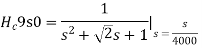
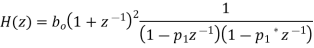
Now find H (z) by first noting that 

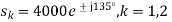
Using the pole/ zero mapping formula
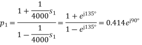
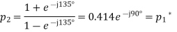
We can now write
Find  by setting
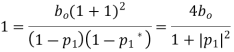
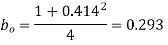
Finally after multiplying out the numerator and denominator we obtain

Compare:
Sr No. | Impulse Invariance | Bilinear Transformation |
1 | In this method IIR filters are designed having a unit sample response h (n) that is sampled version of the impulse response of the analog filter. | This method of IIR filter design is based on the trapezoidal formula for numerical integration. |
2 | The bilinear transformation is a conformal mapping that transforms the j | The bilinear transformation is a conformal mapping tjat transforms the |
3 | For design of LPF, HPF and almost all types of bandpass and band stop filters this method is used. | For designing of LPF, HPF and almost all types of bandpass and band stop filters this method is used. |
4 | Frequency relationship is non –linear. Frequency warping or frequency compression is due to non – linearity. | Frequency relationship is non linear. Frequency warping or frequency compression is due to non – linearity. |
5 | All poles are mapped from s plane to the z plane by the relationship | All poles and zeros are mapped. |


It is also known as Bilinear Transformation method.
The bilinear transform is the result of a numerical integration of the analog transfer function into the digital domain. We can define the bilinear transform as:

Find the bilinear transformation which maps points z =2,1,0 onto the points w=1,0,i.
Ans. Let, 
And, 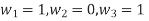
Since bilinear transformation preserves cross ratios,
Thus we have,

Use the bilinear transformation to convert the analog filtrt with system function

 into a digital IIR filter. Select T =0.1
Consider the following system function
Note that the following is the resonant frequency of the analog filter

Consider that the resonant frequency of analog filter must be mapped by selecting the value of parameter
T= 0,1
Use the following mapping for bilinear transformation

Write the system function H(z) of the resultant digital filter

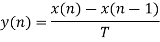
Consider an analog filter. It’s transfer function will be of the differential equation form as shown below.

Taking Laplace transform on both ends:

The transfer function of the analog filter can be given by:
Note that this is just a generic transfer function. To get the transfer function of a digital filter we will dive into some specifics.
Thus,
Taking z-transform on both sides:
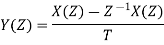
Solving for the transfer function of the digital filter:
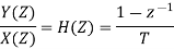
The mapping between S and Z planes
To map from s to z-plane we need to find the values of σ and Ω in s = σ + jΩ. We have the relationship between s and z from above as:

Rewriting the above equation for z:

Substituting s = σ+jΩ in the above equation and solving gives us:
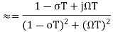
Separating the real and imaginary parts we get:
For σ=0
When we vary Ω from -∞ to +∞, the corresponding locus of points in the z-plane is a circle with radius 1/2 and with its center at z=1/2.
Similarly, when we map the equation  the left half-plane of the s-domain maps inside the circle with 0.5 radians. Moreover, the right half-plane of the s-domain is mapped outside the unit circle.
Mapping of s-plane into the z-plane by the approximation of derivatives method.
Thus we can say that this transformation of an analog filter results in a stable digital filter.
Limitations:
From the above fig, the location of poles in the z-domain is confined to smaller frequencies. Thus the approximation of derivatives method is limited to designing low pass and bandpass IIR filters with small resonant frequencies only. It can’t be used to develop high pass and band-reject filters.
Rounding is a quantization method where we ’round-up’ a particular number to the desired number of bits.
Basically, rounding is the process of reducing the size of a binary number to some desirable finite size. This is done in such a way that the rounded off number is as close to the original unquantized number as possible.
Interestingly, the rounding process is a combination of truncation and addition.
In rounding a number to say b-bits, first, the number is truncated to the desired number of bits. Then depending on the number that existed next to the LSB before truncation, an addition to the LSB is performed.
If that particular number (previously next to the LSB) was 0, then 0 is added to the LSB. If that number was 1, then a 1 is added to the LSB.
Consider the same example as above, suppose we wish to truncate the following 8-bit number to 4-bits.
X = 0.01101011 truncates to X = 0.0110
Since the number next to the current LSB was 1, we add 1 to the current LSB.
Thus X is now 0.0111
Converting both the unquantized and rounded off numbers to decimal, we notice that the magnitude of error is less relative to truncation. (0.01101011 equals 0.418 and 0.0111 equals 0.438).
Thus rounding is preferable than truncation.
The magnitude of error in rounding is given by the formula:

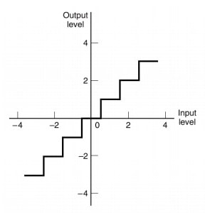
Fig.: Rounding
Digital Signal Processing the computations like FFT algorithm, ADC and filter designs are associated with numbers and coefficients.
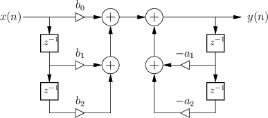
Direct form I
The difference equation


specifies the Direct-Form I (DF-I) implementation of a digital filter. The DF-I signal flow graph for the second-order case is shown in Fig.
Figure : Direct-Form-I implementation of a 2nd-order digital filter. |
Direct form II
The signal flow graph for the Direct-Form-II (DF-II) realization of the second-order IIR filter section is shown in Fig.
Figure : Direct-Form-II implementation of a 2nd-order digital filter. |
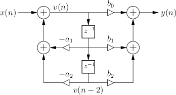
The difference equation for the second-order DF-II structure can be written as


which can be interpreted as a two-pole filter followed in series by a two-zero filter.
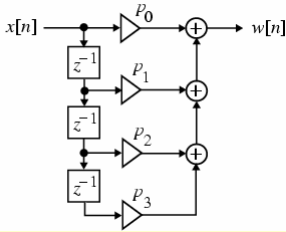
The filter section can be seen to be an FIR filter and can be realized as shown below
W[n] = p0x[n] + p1x[n-1] + p2x[n-2] +p3x[n-3]
The time-domain representation of H2(z) is given by
Y[n] = w[n] –d1y[n-1] –d2y[n-2] – d3y[n-3]
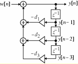
A cascade of the two structures realizing and leads to the realization of shown below and is known as the direct form I structure
Direct form II and cascade form realizations of
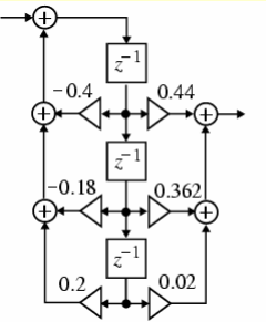
Direct form II
cascade form
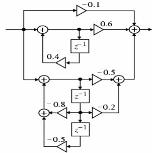
Parallel Form
Example. A partial fraction expansion of
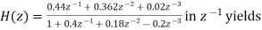
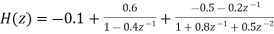
The corresponding parallel form I realization is shown below
References:
1. John G Prokis , “Digital Signal Processing ,Principles, Algorithms and
Application”,PHI
2. S.K.Mitra, “Digital Signal Processing”, TMH
3. E. C. Ifleachor and B. W. Jervis, “Digital Signal Processing- A Practical
Approach”, Second Edition, Pearson education.
4.Avtar Singh, S. Srinivasan, “Digital Signal Processing Implementation using DSP,
Microprocessors with examples from TMS 320C6XXX”, Thomas Publication.


