Unit - 3
Classification & Regression
Decision Tree is a Supervised learning technique that can be used for both classification and Regression problems, but mostly it is preferred for solving Classification problems. It is a tree-structured classifier, where internal nodes represent the features of a dataset, branches represent the decision rules and each leaf node represents the outcome.
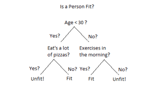
Fig 1: Decision tree example
In a Decision tree can be divided into:
● Decision Node
● Leaf Node
Decision nodes are marked by multiple branches that represent different decision conditions whereas output of those decisions is represented by leaf node and do not contain further branches.
The decision tests are performed on the basis of features of the given dataset.
It is a graphical representation for getting all the possible solutions to a problem/decision based on given conditions.
Decision Tree algorithm:
● Comes under the family of supervised learning algorithms.
● Unlike other supervised learning algorithms, decision tree algorithms can be used for solving regression and classification problems.
● Are used to create a training model that can be used to predict the class or value of the target variable by learning simple decision rules inferred from prior data (training data).
● Can be used for predicting a class label for a record we start from the root of the tree.
● Values of the root attribute are compared with the record’s attribute. On the basis of comparison, a branch corresponding to that value is considered and jumps to the next node.
Issues in Decision tree learning
● It is less appropriate for estimation tasks where the goal is to predict the value of a continuous attribute.
● This learning is prone to errors in classification problems with many classes and relatively small number of training examples.
● This learning can be computationally expensive to train. The process of growing a decision tree is computationally expensive. At each node, each candidate splitting field must be sorted before its best split can be found. In some algorithms, combinations of fields are used and a search must be made for optimal combining weights. Pruning algorithms can also be expensive since many candidate sub-trees must be formed and compared.
- Avoiding overfitting
A decision tree’s growth is specified in terms of the number of layers, or depth, it’s allowed to have. The data available to train the decision tree is split into training and testing data and then trees of various sizes are created with the help of the training data and tested on the test data. Cross-validation can also be used as part of this approach. Pruning the tree, on the other hand, involves testing the original tree against pruned versions of it. Leaf nodes are removed from the tree as long as the pruned tree performs better on the test data than the larger tree.
Two approaches to avoid overfitting in decision trees:
● Allow the tree to grow until it overfits and then prune it.
● Prevent the tree from growing too deep by stopping it before it perfectly classifies the training data.
2. Incorporating continuous valued attributes
3. Alternative measures for selecting attributes
● Prone to overfitting.
● Require some kind of measurement as to how well they are doing.
● Need to be careful with parameter tuning.
● Can create biased learned trees if some classes dominate.
Random forest
Random forest is an ensemble model in which several trees are grown and objects are classified based on the "votes" of all the trees. In other words, an item is allocated to the class with the greatest votes across all trees. The problem of strong bias (overfitting) could be solved this way. (— courtesy of Kaggle)
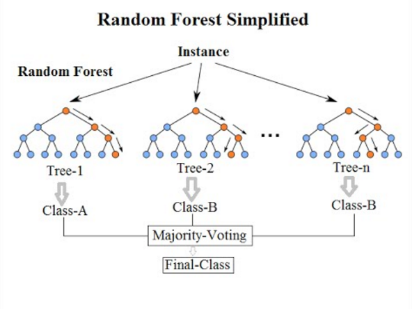
Fig 2: Random forest
The random forest classifier is a meta-estimator that fits a number of decision trees on different sub-samples of datasets and utilises average to improve the model's predictive accuracy and control over-fitting. The size of the sub-sample is always the same as the size of the original input sample, but the samples are generated with replacement.
Pros of RF:
● It can handle big data sets with high dimensionality and produce Importance of Variable, which is useful for data exploration.
● Could deal with missing data and retain accuracy.
Cons of RF:
● Users have limited influence over what the model does, therefore it may be a black box.
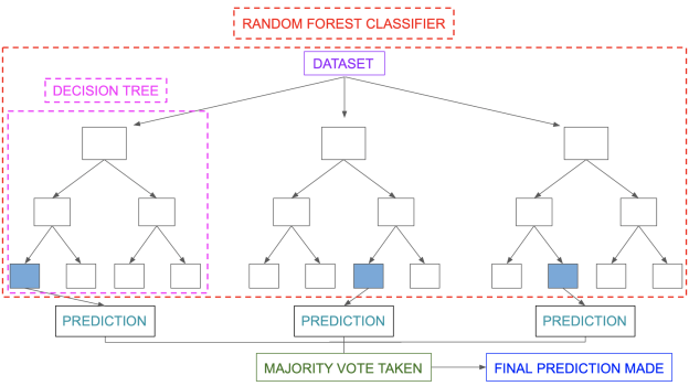
Classification in random forest
Random forest classification uses an ensemble methodology to achieve the desired result. Various decision trees are trained using the training data. This dataset contains observations and features that will be chosen at random when nodes are split.
Various decision trees are used in a rain forest system. There are three types of nodes in a decision tree: decision nodes, leaf nodes, and the root node. Each tree's leaf node represents the final output produced by that particular decision tree. The final product is chosen using a majority-voting procedure. In this situation, the final output of the rain forest system is the output chosen by the majority of decision trees. A simple random forest classifier is depicted in the diagram below.
Key takeaway:
Decision Tree is a Supervised learning technique that can be used for both classification and Regression problems, but mostly it is preferred for solving Classification problems.
It is a tree-structured classifier, where internal nodes represent the features of a dataset, branches represent the decision rules and each leaf node represents the outcome.
The Naïve Bayes algorithm is comprised of two words Naïve and Bayes, Which can be described as:
● Naïve: It is called Naïve because it assumes that the occurrence of a certain feature is independent of the occurrence of other features. Such as if the fruit is identified based on color, shape, and taste, then red, spherical, and sweet fruit is recognized as an apple. Hence each feature individually contributes to identifying that it is an apple without depending on each other.
● Bayes: It is called Bayes because it depends on the principle of Bayes’ Theorem.
Naïve Bayes Classifier Algorithm
Naïve Bayes algorithm is a supervised learning algorithm, which is based on the Bayes theorem and used for solving classification problems. It is mainly used in text classification that includes a high-dimensional training dataset.
Naïve Bayes Classifier is one of the simple and most effective Classification algorithms which help in building fast machine learning models that can make quick predictions.
It is a probabilistic classifier, which means it predicts based on the probability of an Object.
Some popular examples of the Naïve Bayes Algorithm are spam filtration, Sentimental analysis, and classifying articles.
Bayes’ Theorem:
● Bayes’ theorem is also known as Bayes’ Rule or Bayes’ law, which is used to determine the probability of a hypothesis with prior knowledge. It depends on the conditional probability.
● The formula for Bayes’ theorem is given as:
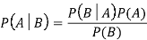
Where,
● P(A|B) is Posterior probability: Probability of hypothesis A on the observed event B.
● P(B|A) is Likelihood probability: Probability of the evidence given that the probability of a hypothesis is true.
● P(A) is Prior Probability: Probability of hypothesis before observing the evidence.
● P(B) is a Marginal Probability: Probability of Evidence.
Working of Naïve Bayes’ Classifier can be understood with the help of the below example:
Suppose we have a dataset of weather conditions and corresponding target variable “Play”. So using this dataset we need to decide whether we should play or not on a particular day according to the weather conditions. So to solve this problem, we need to follow the below steps:
Convert the given dataset into frequency tables.
Generate a Likelihood table by finding the probabilities of given features.
Now, use Bayes theorem to calculate the posterior probability.
Problem: If the weather is sunny, then the Player should play or not?
Solution: To solve this, first consider the below dataset:
Outlook Play
0 Rainy Yes
1 Sunny Yes
2 Overcast Yes
3 Overcast Yes
4 Sunny No
5 Rainy Yes
6 Sunny Yes
7 Overcast Yes
8 Rainy No
9 Sunny No
10 Sunny Yes
11 Rainy No
12 Overcast Yes
13 Overcast Yes
Frequency table for the Weather Conditions:
Weather Yes No
Overcast 5 0
Rainy 2 2
Sunny 3 2
Total 10 5
Likelihood table weather condition:
Weather No Yes
Overcast 0 5 5/14 = 0.35
Rainy 2 2 4/14 = 0.29
Sunny 2 3 5/14 = 0.35
All 4/14=0.29 10/14=0.71
Applying Bayes’ theorem:
P(Yes|Sunny)= P(Sunny|Yes)*P(Yes)/P(Sunny)
P(Sunny|Yes)= 3/10= 0.3
P(Sunny)= 0.35
P(Yes)=0.71
So P(Yes|Sunny) = 0.3*0.71/0.35= 0.60
P(No|Sunny)= P(Sunny|No)*P(No)/P(Sunny)
P(Sunny|NO)= 2/4=0.5
P(No)= 0.29
P(Sunny)= 0.35
So P(No|Sunny)= 0.5*0.29/0.35 = 0.41
So as we can see from the above calculation that P(Yes|Sunny)>P(No|Sunny)
Hence on a Sunny day, the Player can play the game.
Advantages of Naïve Bayes Classifier:
● Naïve Bayes is one of the fast and easy ML algorithms to predict a class of datasets.
● It can be used for Binary as well as Multi-class Classifications.
● It performs well in Multi-class predictions as compared to the other Algorithms.
● It is the most popular choice for text classification problems.
Disadvantages of Naïve Bayes Classifier:
● Naive Bayes assumes that all features are independent or unrelated, so it cannot learn the relationship between features.
Applications of Naïve Bayes Classifier:
● It is used for Credit Scoring.
● It is used in medical data classification.
● It can be used in real-time predictions because Naïve Bayes Classifier is an eager
● learner.
● It is used in Text classification such as Spam filtering and Sentiment analysis.
Types of Naïve Bayes Model:
There are three types of Naive Bayes Model, which are given below:
Gaussian: The Gaussian model assumes that features follow a normal distribution. This means if predictors take continuous values instead of discrete, then the model assumes that these values are sampled from the Gaussian distribution.
Multinomial: The Multinomial Naïve Bayes classifier is used when the data is multinomial distributed. It is primarily used for document classification problems, it means a particular document belongs to which category such as Sports, Politics, education, etc.
The classifier uses the frequency of words for the predictors.
Bernoulli: The Bernoulli classifier works similarly to the Multinomial classifier, but the predictor variables are the independent Booleans variables. Such as if a particular word is present or not in a document. This model is also famous for document classification tasks.
Key takeaway
Naïve Bayes algorithm is a supervised learning algorithm, which is based on the Bayes theorem and used for solving classification problems.
Naïve Bayes Classifier is one of the simple and most effective Classification algorithms which help in building fast machine learning models that can make quick predictions.
Bayes’ theorem is also known as Bayes’ Rule or Bayes’ law, which is used to determine the probability of a hypothesis with prior knowledge.
SVM is another linear classification algorithm (One which separates data with a hyperplane) just like logistic regression and perceptron algorithms.
Given any linearly separable data, we can have multiple hyperplanes that can function as a separation boundary as shown. SVM selects the "optimal" hyperplane of all candidate hyperplanes.
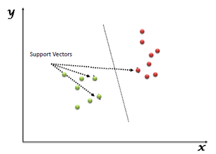
Fig 3: Support vector machine
To understand definition of "optimal" hyperplane, let us first define some concepts we will use
● Margin: It is the distance of the separating hyperplane to its nearest point/points.
● Support Vectors: The point/points closest to the dividing hyperplane.
The optimal hyperplane is defined as the one which maximises the margin. Thus SVM is posed as an optimization problem where we have to maximise margin subject to the constraint that all points lie on the correct side of the separating hyperplane
If all candidate hyperplanes correctly classify the data, why is maximum margin hyperplane the optimal one? One intuitive explanation is - If the incoming samples to be classified contain noise, we do not want them to cross the boundary and be classified incorrectly.
Advantages:
● It works very well with a clear margin of separation
● It is useful in high dimensional spaces.
● It is useful in situations where the number of dimensions is greater than the number of samples.
● It uses a subset of training points in the decision function (called support vectors), so it is also memory efficient.
Disadvantages:
● It doesn’t work well when we have a broad data set because the necessary training time is higher.
● It also doesn’t work very well, when the data set has more noise i.e. target classes are overlapping.
● SVM doesn’t explicitly have probability estimates, these are determined using a costly five-fold cross-validation.
Another approach to linear classification is the logistic regression model, which, despite its name, is a classification rather than a regression system.
In Logistic regression, we take a weighted linear combination of input features and pass it through a sigmoid function which outputs a number between 1 and 0. Unlike perceptron, which only tells us which side of the plane the point lies on, logistic regression gives a likelihood of a point lying on a particular side of the plane.
The probability of classification would be very similar to 1 or 0 as the point goes far away from the plane. The chance of classification of points very close to the plane is close to 0.5.
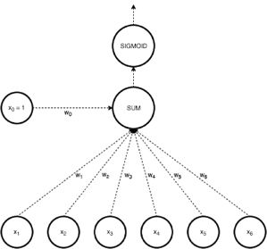
Fig 4: Logistic regression
The model is defined in terms of K-1 log-odds ratios, with an arbitrary class chosen as reference class (in this example it is the last class, K) (in this example it is the last class, K). Consequently, the difference between log-probabilities of belonging to a given class and to the reference class is modelled linearly as
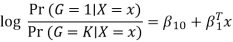
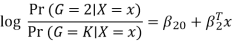
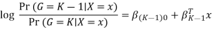
Where G stands for the real, observed class. From here, the probabilities of an observation belonging to each of the groups can be determined as
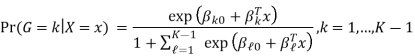
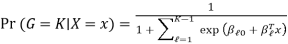
That clearly shows that all class probabilities add up to one.
Logistic regression models are usually calculated by maximum likelihood. Much as linear models for regression can be regularised to increase accuracy, so can logistic regression. In reality, L2 penalty is the default setting. It also supports L1 and Elastic Net penalties (to read more on these, check out the link above), but not all of them are supported by all solvers.
Key takeaway:
● Logistic Regression models the probabilities of an observation belonging to each of the classes through linear functions.
● It is usually considered safer and more stable than discriminant analysis methods, since it is relying on less assumptions.
● It also turned out to be the most accurate for our example spam results.
Support Vector Regression (SVR) is a regression technique that uses the same principles as SVM. Let's take a few moments to grasp the concept of SVR.
The Idea Behind Support Vector Regression
On the basis of a training sample, the aim of regression is to identify a function that approximates mapping from an input domain to real numbers. So let's take a closer look at how SVR truly works.
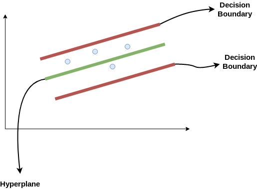
Consider the decision boundary to be these two red lines, and the hyperplane to be the green line. When we move forward with SVR, our goal is to essentially consider the points that are within the decision boundary line. The hyperplane with the most points is the greatest fit line for us.
The first thing we'll figure out is what the decision boundary is (that dangerous red line up there!). Consider these lines to be at any distance from the hyperplane, say 'a'. So, at distances '+a' and '-a' from the hyperplane, we draw these lines. Epsilon is the name given to this 'a' in the text.
Assume that the hyperplane's equation is as follows:
Y = wx+b (equation of hyperplane)
The decision boundary equations then become:
Wx+b= +a
Wx+b= -a
As a result, every hyperplane that fulfils our SVR must satisfy the following conditions:
-a < Y- wx+b < +a
The key goal here is to choose a decision boundary that is 'a' distance from the original hyperplane and contains data points or support vectors that are closest to the hyperplane.
As a result, we'll only consider points that fall within the decision boundary and have the lowest mistake rate, or those that fall within the Margin of Tolerance. This results in a more accurate model.
- Decision Tree is a Supervised learning technique that can be used for both classification and Regression problems, but mostly it is preferred for solving Classification problems. It is a tree-structured classifier, where internal nodes represent the features of a dataset, branches represent the decision rules and each leaf node represents the outcome.
- In a Decision tree, there are two nodes, which are the Decision Node and Leaf Node. Decision nodes are used to make any decision and have multiple branches, whereas Leaf nodes are the output of those decisions and do not contain any further branches.
- The decisions or the test are performed on the basis of features of the given dataset.
It is a graphical representation for getting all the possible solutions to a problem/decision based on given conditions.
- It is called a decision tree because, similar to a tree, it starts with the root node, which expands on further branches and constructs a tree-like structure.
- In order to build a tree, we use the CART algorithm, which stands for Classification and Regression Tree algorithm.
- A decision tree simply asks a question, and based on the answer (Yes/No), it further split the tree into subtrees.
- Below diagram explains the general structure of a decision tree:
Note: A decision tree can contain categorical data (YES/NO) as well as numeric data.
Why use Decision Trees?
There are various algorithms in Machine learning, so choosing the best algorithm for the given dataset and problem is the main point to remember while creating a machine learning model. Below are the two reasons for using the Decision tree:
- Decision Trees usually mimic human thinking ability while making a decision, so it is easy to understand.
- The logic behind the decision tree can be easily understood because it shows a tree-like structure.
Decision Tree Terminologies
● Root Node: Root node is from where the decision tree starts. It represents the entire dataset, which further gets divided into two or more homogeneous sets.
● Leaf Node: Leaf nodes are the final output node, and the tree cannot be segregated further after getting a leaf node.
● Splitting: Splitting is the process of dividing the decision node/root node into sub-nodes according to the given conditions.
● Branch/Sub Tree: A tree formed by splitting the tree.
● Pruning: Pruning is the process of removing the unwanted branches from the tree.
● Parent/Child node: The root node of the tree is called the parent node, and other nodes are called the child nodes.
How does the Decision Tree algorithm Work?
In a decision tree, for predicting the class of the given dataset, the algorithm starts from the root node of the tree. This algorithm compares the values of root attribute with the record (real dataset) attribute and, based on the comparison, follows the branch and jumps to the next node.
For the next node, the algorithm again compares the attribute value with the other sub-nodes and move further. It continues the process until it reaches the leaf node of the tree. The complete process can be better understood using the below algorithm:
Step-1: Begin the tree with the root node, says S, which contains the complete dataset.
Step-2: Find the best attribute in the dataset using Attribute Selection Measure (ASM).
Step-3: Divide the S into subsets that contains possible values for the best attributes.
Step-4: Generate the decision tree node, which contains the best attribute.
Step-5: Recursively make new decision trees using the subsets of the dataset created in step -3. Continue this process until a stage is reached where you cannot further classify the nodes and called the final node as a leaf node.
Example: Suppose there is a candidate who has a job offer and wants to decide whether he should accept the offer or not. So, to solve this problem, the decision tree starts with the root node (Salary attribute by ASM). The root node splits further into the next decision node (distance from the office) and one leaf node based on the corresponding labels. The next decision node further gets split into one decision node (Cab facility) and one leaf node. Finally, the decision node splits into two leaf nodes (Accepted offers and Declined offer). Consider the below diagram:
Attribute Selection Measures
While implementing a Decision tree, the main issue arises that how to select the best attribute for the root node and for sub-nodes. So, to solve such problems there is a technique which is called as Attribute selection measure or ASM. By this measurement, we can easily select the best attribute for the nodes of the tree. There are two popular techniques for ASM, which are:
- Information Gain
- Gini Index
1. Information Gain:
- Information gain is the measurement of changes in entropy after the segmentation of a dataset based on an attribute.
- It calculates how much information a feature provides us about a class.
- According to the value of information gain, we split the node and build the decision tree.
- A decision tree algorithm always tries to maximize the value of information gain, and a node/attribute having the highest information gain is split first. It can be calculated using the below formula:
1. Information Gain= Entropy(S)- [(Weighted Avg) *Entropy(each feature)
Entropy: Entropy is a metric to measure the impurity in a given attribute. It specifies randomness in data. Entropy can be calculated as:
Entropy(s)= -P(yes)log2 P(yes)- P(no) log2 P(no)
Where,
- S= Total number of samples
- P(yes)= probability of yes
- P(no)= probability of no
2. Gini Index:
- Gini index is a measure of impurity or purity used while creating a decision tree in the CART(Classification and Regression Tree) algorithm.
- An attribute with the low Gini index should be preferred as compared to the high Gini index.
- It only creates binary splits, and the CART algorithm uses the Gini index to create binary splits.
- Gini index can be calculated using the below formula:
Gini Index= 1- ∑jPj2
Pruning: Getting an Optimal Decision tree
Pruning is a process of deleting the unnecessary nodes from a tree in order to get the optimal decision tree.
A too-large tree increases the risk of overfitting, and a small tree may not capture all the important features of the dataset. Therefore, a technique that decreases the size of the learning tree without reducing accuracy is known as Pruning. There are mainly two types of trees pruning technology used:
- Cost Complexity Pruning
- Reduced Error Pruning.
Advantages of the Decision Tree
- It is simple to understand as it follows the same process which a human follow while making any decision in real-life.
- It can be very useful for solving decision-related problems.
- It helps to think about all the possible outcomes for a problem.
- There is less requirement of data cleaning compared to other algorithms.
Disadvantages of the Decision Tree
- The decision tree contains lots of layers, which makes it complex.
- It may have an overfitting issue, which can be resolved using the Random Forest algorithm.
- For more class labels, the computational complexity of the decision tree may increase.
Python Implementation of Decision Tree
Now we will implement the Decision tree using Python. For this, we will use the dataset "user_data.csv," which we have used in previous classification models. By using the same dataset, we can compare the Decision tree classifier with other classification models such as KNN SVM, Logistic Regression, etc.
Steps will also remain the same, which are given below:
- Data Preprocessing step
- Fitting a Decision-Tree algorithm to the Training set
- Predicting the test result
- Test accuracy of the result(Creation of Confusion matrix)
- Visualizing the test set result.
1. Data Preprocessing Step:
Below is the code for the pre-processing step:
- # importing libraries
- Import numpy as nm
- Import matplotlib.pyplot as mtp
- Import pandas as pd
- #importing datasets
- Data_set= pd.read_csv('user_data.csv')
- #Extracting Independent and dependent Variable
- x= data_set.iloc[:, [2,3]].values
- y= data_set.iloc[:, 4].values
- # Splitting the dataset into training and test set.
- From sklearn.model_selection import train_test_split
- x_train, x_test, y_train, y_test= train_test_split(x, y, test_size= 0.25, random_state=0)
- #feature Scaling
- From sklearn.preprocessing import StandardScaler
- St_x= StandardScaler()
- x_train= st_x.fit_transform(x_train)
- x_test= st_x.transform(x_test)
2. Fitting a Decision-Tree algorithm to the Training set
Now we will fit the model to the training set. For this, we will import the DecisionTreeClassifier class from sklearn.tree library. Below is the code for it:
- #Fitting Decision Tree classifier to the training set
- From sklearn.tree import DecisionTreeClassifier
- Classifier= DecisionTreeClassifier(criterion='entropy', random_state=0)
- Classifier.fit(x_train, y_train)
In the above code, we have created a classifier object, in which we have passed two main parameters;
- "criterion='entropy': Criterion is used to measure the quality of split, which is calculated by information gain given by entropy.
- Random_state=0": For generating the random states.
Below is the output for this:
Out[8]:
DecisionTreeClassifier(class_weight=None, criterion='entropy', max_depth=None,
Max_features=None, max_leaf_nodes=None,
Min_impurity_decrease=0.0, min_impurity_split=None,
Min_samples_leaf=1, min_samples_split=2,
Min_weight_fraction_leaf=0.0, presort=False,
Random_state=0, splitter='best')
3. Predicting the test result
Now we will predict the test set result. We will create a new prediction vector y_pred. Below is the code for it:
- #Predicting the test set result
- y_pred= classifier.predict(x_test)
Output:
In the below output image, the predicted output and real test output are given. We can clearly see that there are some values in the prediction vector, which are different from the real vector values. These are prediction errors.
4. Test accuracy of the result (Creation of Confusion matrix)
In the above output, we have seen that there were some incorrect predictions, so if we want to know the number of correct and incorrect predictions, we need to use the confusion matrix. Below is the code for it:
- #Creating the Confusion matrix
- From sklearn.metrics import confusion_matrix
- Cm= confusion_matrix(y_test, y_pred)
5. Visualizing the training set result:
Here we will visualize the training set result. To visualize the training set result we will plot a graph for the decision tree classifier. The classifier will predict yes or No for the users who have either Purchased or Not purchased the SUV car as we did in Logistic Regression. Below is the code for it:
- #Visualizing the training set result
- From matplotlib.colors import ListedColormap
- x_set, y_set = x_train, y_train
- x1, x2 = nm.meshgrid(nm.arange(start = x_set[:, 0].min() - 1, stop = x_set[:, 0].max() + 1, step =0.01),
- Nm.arange(start = x_set[:, 1].min() - 1, stop = x_set[:, 1].max() + 1, step = 0.01))
- Mtp.contourf(x1, x2, classifier.predict(nm.array([x1.ravel(), x2.ravel()]).T).reshape(x1.shape),
- Alpha = 0.75, cmap = ListedColormap(('purple','green' )))
- Mtp.xlim(x1.min(), x1.max())
- Mtp.ylim(x2.min(), x2.max())
- Fori, j in enumerate(nm.unique(y_set)):
- Mtp.scatter(x_set[y_set == j, 0], x_set[y_set == j, 1],
- c = ListedColormap(('purple', 'green'))(i), label = j)
- Mtp.title('Decision Tree Algorithm (Training set)')
- Mtp.xlabel('Age')
- Mtp.ylabel('Estimated Salary')
- Mtp.legend()
- Mtp.show()
6. Visualizing the test set result:
Visualization of test set result will be similar to the visualization of the training set except that the training set will be replaced with the test set.
- #Visualizing the test set result
- From matplotlib.colors import ListedColormap
- x_set, y_set = x_test, y_test
- x1, x2 = nm.meshgrid(nm.arange(start = x_set[:, 0].min() - 1, stop = x_set[:, 0].max() + 1, step =0.01),
- Nm.arange(start = x_set[:, 1].min() - 1, stop = x_set[:, 1].max() + 1, step = 0.01))
- Mtp.contourf(x1, x2, classifier.predict(nm.array([x1.ravel(), x2.ravel()]).T).reshape(x1.shape),
- Alpha = 0.75, cmap = ListedColormap(('purple','green' )))
- Mtp.xlim(x1.min(), x1.max())
- Mtp.ylim(x2.min(), x2.max())
- Fori, j in enumerate(nm.unique(y_set)):
- Mtp.scatter(x_set[y_set == j, 0], x_set[y_set == j, 1],
- c = ListedColormap(('purple', 'green'))(i), label = j)
- Mtp.title('Decision Tree Algorithm(Test set)')
- Mtp.xlabel('Age')
- Mtp.ylabel('Estimated Salary')
- Mtp.legend()
- Mtp.show()
Random forest
A random forest is a machine learning technique for solving classification and regression problems. It makes use of ensemble learning, which is a technique for solving complicated problems by combining several classifiers.
Many decision trees make up a random forest algorithm. Bagging or bootstrap aggregation are used to train the 'forest' formed by the random forest method. Bagging is a meta-algorithm that increases the accuracy of machine learning methods by grouping them together.
The (random forest) algorithm determines the outcome based on decision tree predictions. It forecasts by averaging or averaging the output of various trees. The precision of the result improves as the number of trees grows.
A random forest method overcomes the drawbacks of a decision tree algorithm. It reduces dataset overfitting and improves precision. It generates forecasts without requiring a large number of package setups (like scikit-learn).
Features of a Random Forest Algorithm
● It outperforms the decision tree algorithm in terms of accuracy.
● It is a useful tool for dealing with missing data.
● Without hyper-parameter adjustment, it can provide a reasonable prediction.
● It overcomes the problem of decision tree overfitting.
● At the node's splitting point in every random forest tree, a subset of features is chosen at random.
Regression in random forest
The other duty that a random forest algorithm does is regression. The principle of simple regression is followed by a random forest regression. In the random forest model, the values of dependent (features) and independent variables are passed.
Random forest regressions can be performed in a variety of systems, including SAS, R, and Python. Each tree in a random forest regression makes a unique prediction. The regression's output is the average prediction of the individual trees. This is in contrast to random forest classification, which determines the output based on the decision trees' class mode.
Although the concepts of random forest regression and linear regression are similar, their functions differ. y=bx + c is the formula for linear regression, where y is the dependent variable, x is the independent variable, b is the estimation parameter, and c is a constant. A sophisticated random forest regression's function is similar to that of a blackbox.
K-Means Clustering is an unsupervised learning approach used in machine learning and data science to solve clustering problems. K specifies the number of predefined clusters that must be produced during the process; for example, if K=2, two clusters will be created, and if K=3, three clusters will be created, and so on.
It allows us to cluster data into different groups and provides a simple technique to determine the categories of groups in an unlabeled dataset without any training.
It's a centroid-based approach, which means that each cluster has its own centroid. The main goal of this technique is to reduce the sum of distances between data points and the clusters that they belong to.
For numeric results, K-Means clustering is one of the most commonly used prototype-based clustering algorithms. The centroid or mean of all the data points in a cluster is the prototype of a cluster in k-means. As a consequence, the algorithm works best with continuous numeric data. When dealing with data that includes categorical variables or a mixture of quantitative and categorical variables.
The technique takes an unlabeled dataset as input, separates it into a k-number of clusters, and continues the procedure until no better clusters are found. In this algorithm, the value of k should be predetermined.
The k-means clustering algorithm primarily accomplishes two goals:
● Iteratively determines the optimal value for K centre points or centroids.
● Each data point is assigned to the k-center that is closest to it. A cluster is formed by data points that are close to a specific k-center.
As a result, each cluster contains datapoints with certain commonality and is isolated from the others.
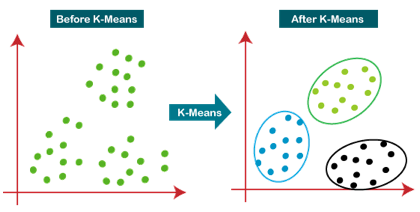
Fig 5: Working of the K-means Clustering Algorithm
Pseudo Algorithm
- Choose an appropriate value of K (number of clusters we want)
- Generate K random points as initial cluster centroids
- Until convergence (Algorithm converges when centroids remain the same between iterations):
● Assign each point to a cluster whose centroid is nearest to it ("Nearness" is measured as the Euclidean distance between two points)
● Calculate new values of centroids of each cluster as the mean of all points assigned to that cluster
Advantages
Some of the benefits of K-Means clustering techniques are as follows:
● It is simple to comprehend and implement.
● K-means would be faster than Hierarchical clustering if we had a high number of variables.
● An instance can modify the cluster when centroids are recalculated.
● When compared to Hierarchical clustering, K-means produces tighter groupings.
Disadvantages
Some of the drawbacks of K-Means clustering techniques are as follows:
● The number of clusters, or the value of k, is difficult to anticipate.
● Initial inputs such as the number of clusters have a significant impact on output (value of k).
● The order in which the data is entered will have a significant impact on the final result.
● It is very sensitive to rescaling. If we will rescale our data by means of normalization or standardization, then the output will completely change.
● It is not good in doing clustering job if the clusters have a complicated geometric shape.
Key takeaway
● K-Means clustering is one of the most commonly used prototype-based clustering algorithms.
● The algorithm works best with continuous numeric data.
● When dealing with data that includes categorical variables or a mixture of quantitative and categorical variables.
● K-Means is a more effective algorithm. Defining distances between each diamond takes longer than computing a mean.
- It is one of the simplest Machine Learning algorithms based on Supervised Learning technique.
- Algorithm assumes the similarity between the new case/data and available cases, puts the new case into the category that is most similar to the available categories.
- Algorithm stores all the available data and classifies a new data point based on the similarity. This means when new data appears then it can be easily classified into a well suite category by using K NN algorithm.
- Algorithm can be used for Regression and Classification but mostly it is used for the Classification type problems.
- It is a non-parametric algorithm, which means it does not make any assumption on underlying data.
- It is known as lazy learner algorithm because it does not learn from the training set immediately instead it stores the dataset and at the time of classification, it performs an action on the dataset.
- Algorithm at the training phase just stores the dataset and when it gets new data, then it classifies that data into a category that is much similar to the new data.
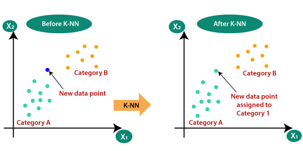
Importance of KNN Algorithm
Consider there are 2 categories, that is Category A and Category B, and we have a new data point x1, so this data point will lie in which of these categories. To solve this type of problem, we need algorithm. With the help of algorithm, we can easily identify the category or class of a particular dataset. Consider the below diagram.
The K-NN working can be explained on the basis of the below algorithm.
Step-1: Select the number K of the neighbors
Step-2: Calculate the Euclidean distance of K number of neighbors
Step-3: Take the K nearest neighbors as per the calculated Euclidean distance.
Step-4: Among these k neighbors, count the number of the data points in each category.
Step-5: Assign the new data points to that category for which the number of the neighbor is maximum.
Step-6: Our model is ready.
Sentiment Analysis
Sentiment analysis is a machine learning text analysis technique that assigns sentiment (opinion, feeling, or emotion) to individual words or full texts on a polarity scale of Positive, Negative, or Neutral.
It can read thousands of pages in minutes or keep an eye on your social media accounts for posts about you. For example, in the tweet below about the messaging tool Slack, all of the individual sentences would be categorised as Positive. Companies can now track product launches and marketing efforts in real time to observe how customers react.
Sentiment analysis models may be trained to read for things like sarcasm and misused or misspelt phrases using powerful machine learning methods. Models, once correctly trained, can consistently give accurate results in a fraction of the time it takes humans.
Try out Monkey Learn's pretrained sentiment classification tool right away. Alternatively, discover how to tailor your own sentiment classifier to your company's language and needs.
Email Spam Classification
Email spam categorization is one of the most prevalent uses of classification since it works nonstop and requires minimal human intervention. It saves us from laborious deletion jobs and, in some cases, costly phishing frauds.
The various algorithms are used by email apps to determine if an email is intended for the recipient or is unwanted spam. Spam emails are weeded out of the ordinary inbox using text analysis categorization techniques: perhaps a recipient's name is misspelt, or certain scamming phrases are utilised.
As we've all experienced when signing up for an email list that ends up in the spam bin, spam classifiers still need to be trained to some extent.
Document Classification
Document categorization is the process of categorising documents based on their content. Previously, this was done manually, such as in library sciences or with hand-ordered legal files. Machine learning classification techniques, on the other hand, make this possible.
Document classification varies from text classification in that it classifies entire documents rather than individual words or phrases. When using online search engines, cross-referencing themes in legal documents, and examining healthcare records by drug and illness, this is put into effect.
Image Classification
A given image is assigned to previously trained categories through image classification. These could be the image's subject, a numerical value, or a theme, for example. Multi-label image classifiers, which work similarly to multi-label text classifiers, can be used to tag an image of a stream into different labels, such as "stream," "water," "outdoors," and so on.
You can tag photographs to train your model for appropriate categories using supervised learning methods. The more you train it, the better it will work, just like any other machine learning model.
References:
- Stuart Russell and Peter Norvig (1995), “Artificial Intelligence: A Modern Approach,” Third edition, Pearson, 2003.
- Solanki, Kumar, Nayyar, Emerging Trends and Applications of Machine Learning, IGI Global, 2018.
- B Joshi, Machine Learning and Artificial Intelligence, Springer, 2020.
- Mohri, Rostamizdeh, Talwalkar, Foundations of Machine Learning, MIT Press, 2018.


