Unit - 2
Feature Extraction and Selection
Feature extraction is a dimensionality reduction procedure that reduces a large set of raw data into smaller groupings for processing. The enormous number of variables in these large data sets necessitates a lot of computational resources to process. Feature extraction refers to strategies for selecting and/or combining variables into features in order to reduce the amount of data that needs to be processed while still accurately and thoroughly characterising the original data set.
Why is this Useful?
When you need to reduce the number of resources needed for processing without losing significant or relevant information, feature extraction comes in handy. Feature extraction can also help to reduce the amount of redundant data in a study. Furthermore, the reduction of data and the machine's efforts in constructing variable combinations (features) speed up the learning and generalisation stages of the machine learning process.
Statistical
Statistics enables us to evaluate both quantitative and qualitative data in a reasonably quick and simple manner. In previous chapters, we used statistical measures to get new insight and perspective on our data, especially, we identified mean and standard deviation as metrics that allowed us to construct z-scores and scale our data.
A statistical test is a method of determining whether a random variable follows the null hypothesis or the alternate hypothesis. It basically shows you whether there are substantial differences between the sample and the population, or between two or more samples. For this, you can utilise descriptive statistics like mean, median, mode, range, or standard deviation. The mean, on the other hand, is what we usually use. A number is generated by the statistical test, which is then compared to the p-value. If it is greater than the p-value, the null hypothesis is accepted; otherwise, it is rejected.
The following is the technique for implementing each statistical test:
● We use a mathematical procedure to calculate the statistic value.
● The critical value is then calculated using statistical tables.
● The p-value is calculated with the help of critical value.
● If the p-value is greater than 0.05, we accept the null hypothesis; otherwise, we reject it.
In this tutorial, we'll use two new concepts to assist us in choosing features:
● Pearson correlations
● hypothesis testing
Both of these methods are known as univariate feature selection methods, which means that they are quick and convenient when the problem is to select single features at a time to improve the dataset for our machine learning pipeline.
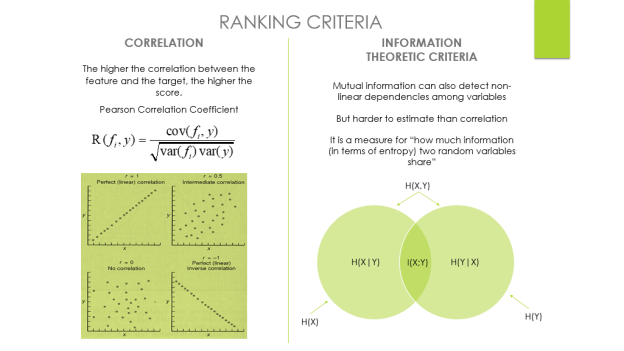
Pearson correlations
The linear link between columns is measured using the Pearson correlation coefficient (which is the default for pandas). The coefficient's value ranges from -1 to +1, with 0 implying that there is no association between them. Closer correlations to -1 or +1 indicate a very strong linear relationship.
It's worth mentioning that Pearson's correlation assumes that each column has a normal distribution (which we are not assuming). Because our dataset is so vast, we can essentially ignore this restriction (over 500 is the threshold).
Hypothesis testing
Hypothesis testing is a statistical tool that allows for more sophisticated statistical examination of particular properties. Feature selection using hypothesis testing, like our own correlation chooser, will attempt to select only the best features from a dataset, but these tests rely on more formalised statistical procedures and are interpreted using p-values.
A hypothesis test is a statistical test that determines whether a condition can be applied to an entire population based on a data sample. A hypothesis test's outcome tells us whether we should believe the hypothesis or reject it in favour of another. A hypothesis test evaluates whether or not to reject the null hypothesis based on sample data from a population. To reach this conclusion, we commonly utilise a p-value (a non-negative decimal with an upper bound of 1 based on our significance level).
The hypothesis we want to test in the instance of feature selection is something like this: True or false: The answer variable is unaffected by this feature. We want to see if this hypothesis holds true for each feature and if the features have any bearing on the response prediction. This is how we dealt with the correlation logic in some ways.
We simply claimed that if the connection between a column and the response is too weak, the supposition that the characteristic has no relevance is correct. If the correlation coefficient is high enough, we can rule out the hypothesis that the characteristic has no importance in favour of the alternative hypothesis that the feature does.
Principal Component Analysis is a feature extraction process in which we generate new independent features from old features and retain only the features that are most relevant in predicting the target from the combination of both. New features are derived from old features, and any function that is less reliant on the target variable can be dropped.
Principal Component Analysis (PCA) is a common technique for reducing the dimensionality of a large data set. Reducing the number of components or features compromises some precision, but it simplifies, examines, and visualizes a broad data set.
It also reduces the model's computational complexity, allowing machine learning algorithms to run faster. It is still a challenge and a point of contention as to how much precision is lost in order to achieve a less complex and reduced-dimension data set. We don't have a fixed answer for this, but when selecting the final set of components, we try to retain as much variation as possible.
Steps involved in PCA
● Ensure that the data is standardized. (where the mean is 0 and the variance is 1)
● Calculate the dimension's covariance matrix.
● From the covariance matrix, obtain the Eigenvectors and Eigenvalues (we can also use correlation matrices or even Single value decomposition ).
● Choose the top k Eigenvectors that correspond to the k largest eigenvalues (k will become the number of dimensions of the new function subspace kd, d is the number of original dimensions) by sorting eigenvalues in descending order.
● Create the projection matrix W using the k Eigenvectors you've chosen.
● To get the new k-dimensional function subspace Y, transform the original data set X through W.
Performance issues
● PCA's potency is directly proportional to the scale of the attributes. If the variables are on different scales, PCA will choose the one with the highest attributes without regard for correlation.
● If the scale of a variable is changed, PCA can change.
● PCA can be difficult to interpret due to the presence of discrete data.
● The appearance of skew in the data with long thick tails can affect the effectiveness of PCA.
● When the relationships between attributes are not linear, PCA is ineffective.
Advantages
● Due to the orthogonal elements, there is a lack of data redundancy.
● Noise reduction due to the use of the maximum variance basis, which automatically eliminates minor variations in the context.
Disadvantages
● It's difficult to do a thorough assessment of covariance.
● The PCA would not be able to capture even the most basic invariance unless the training data specifically provided this detail.
Key takeaway:
Principal Component Analysis (PCA) is a statistical procedure that converts a set of correlated variables into a set of uncorrelated variables using an orthogonal transformation.
PCA is a popular tool for exploratory data analysis and predictive modeling in machine learning.
PCA is also an unsupervised statistical technique for examining the interrelationships between a set of variables.
Adding features to your dataset might help your machine learning model perform better, especially if the model is too simplistic to suit the present data. However, it's critical to concentrate on features that are relevant to the problem you're seeking to solve rather than ones that make no difference. If you're trying to predict flight delays, for example, today's temperature is essential, but three months ago's temperature isn't.
Without losing accuracy, good feature selection removes irrelevant or superfluous columns from your dataset. Unlike dimensionality reduction, feature selection does not entail the creation of new features or the transformation of existing ones; rather, it entails the removal of those that do not contribute value to your research.
By subsetting the original features and shortlisting the best ones with the highest predictive power, feature selection seeks to reduce the size of the original dataset. We can make an informed decision about which feature selection approach will work best for us, but in actuality, working through examples of each method and evaluating the performance of the resulting pipeline is a highly valid way of working in this domain.
The process of picking the characteristics that are relevant to a machine learning model is known as feature selection. It means you only select attributes that have a major impact on the model's output.
Consider what happens when you go grocery shopping at a department store. A product has a lot of data, such as the product name, category, expiration date, MRP, ingredients, and manufacturing information. All of this information pertains to the product's features. Before buying a product, you usually examine the brand, MRP, and expiration date. The section on ingredients and manufacture, on the other hand, is not your affair. As a result, the brand, MRP, and expiry date are important elements, whereas the ingredient and manufacturing data are not. This is how you choose your features.
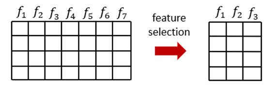
Fig: Illustration of feature selection and data size reduction in tabular data
Importance
The following are some of the advantages of feature selection for machine learning:
● Lowering the risk of overfitting
● Increasing algorithm run speed by lowering the number of operations required to read and preprocess data and execute data science on the production system by lowering the CPU, I/O, and RAM load.
● By disclosing the most informative aspects driving the model's outcomes, the model's interpretability is improved.
Ranking
The technique of ordering features by the value of some scoring function, which commonly gauges feature-relevance, is known as variable ranking.
The score S(fi), which measures some criteria of feature fi, is computed from the training data. A high score, by tradition, indicates a useful (important) trait.
Selecting the k highest ranked features according to S is a simple method for feature selection utilising variable ranking. This is rarely ideal, but it is frequently superior to other, more complicated ways. It is computationally efficient because all that is required is the calculation and sorting of n scores.
Ranking Criteria: Correlation Criteria and Information Theoretic Criteria
Variable Ranking — Single Variable Classifiers
Idea: Choose variables based on their individual prediction ability.
Criteria - The performance of a classifier with only one variable, such as the variable's value.
The error rate is commonly used to measure predictive power (or criteria using False Positive Rate, False Negative Rate)
Ensemble methods (boosting,...) can also be used to deploy a combination of SVCs.
The uncertainty in our dataset or measure of disorder is referred to as entropy. Let me provide an example to try to convey what I'm talking about.
Assume you have a group of friends who decide on a Sunday movie to watch together. There are 2 choices for movies, one is “Lucy” and the second is “Titanic” and now everyone has to tell their choice. After everyone has voted, we notice that "Lucy" receives 4 votes and "Titanic" receives 5 votes. What movie are we going to watch right now? Isn't it difficult to pick only one movie given that the votes for both films are nearly equal?
This is exactly what we term chaos: both movies have an identical number of votes, and we can't pick which one to watch. It would have been a lot easier if "Lucy" received 8 votes and "Titanic" received 2. We may easily conclude that "Lucy" has received the majority of votes, and that everyone will be watching it.
The output of a decision tree is mostly "yes" or "no."
The following is the Entropy formula:

Here p+ is the probability of positive class
p– is the probability of negative class
S is the subset of the training example
How do Decision Trees use Entropy?
Now that we know what entropy is and how to calculate it, we need to understand how it works in this method.
The impurity of a node is measured by entropy. The degree of randomness, or impurity, indicates how unpredictable our data is. A pure sub-split indicates that you should receive either "yes" or "no" as a response.
If a feature starts out with 8 "yes" and 4 "no," after the first split, the left node gets 5 "yes" and 2 "no," while the right node gets 3 "yes" and 2 "no."
Why is it that the split is not pure here? Because some negative classes can still be found in both nodes. To build a decision tree, we must first calculate the impurity of each split, and then make it a leaf node when the purity is 100 percent.
We will use the Entropy formula to determine the impurity of features 2 and 3.
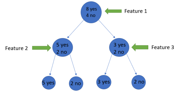
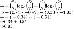
For feature 3
We can observe from the tree that the left node has lower entropy or purity than the right node since the left node has more "yes" and it is easier to decide here.
Always keep in mind that the greater the Entropy, the lower the purity and the greater the impurity.
As previously stated, the goal of machine learning is to reduce uncertainty or impurity in a dataset; in this case, we are obtaining the impurity of a particular node by using entropy; however, we have no way of knowing whether the parent entropy or the entropy of a particular node has decreased or not.
For this, we introduce a new statistic called "Information gain," which indicates how much the parent entropy has dropped after being split with a feature.
Information Gain
Information gain is a decisive factor in which attribute should be chosen as a decision node or root node since it reduces uncertainty when given a feature.
Information gain = E (Y) – E (Y|X)
It's simply the entropy of the entire dataset multiplied by the entropy of the dataset multiplied by some feature.
Consider the following scenario to better comprehend this:
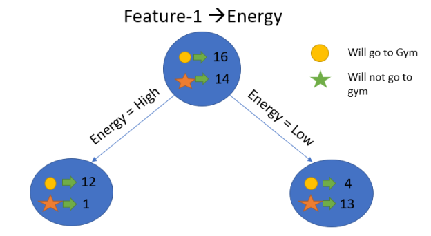
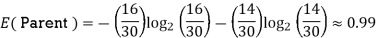
Assume that our entire population has 30 instances. The goal of the dataset is to forecast whether or not a person will go to the gym. Let's pretend that 16 people go to the gym and 14 don't.
Feature 1 is “Energy” which takes two values “high” and “low”
Feature 2 is “Motivation” which takes 3 values “No motivation”, “Neutral” and “Highly motivated”.
Let's look at how these two features will be used to create our decision tree. Information gain will be used to determine which feature should be the root node and which should be placed after the split.
Calculate entropy


We'll do the following to see each node's weighted average entropy:
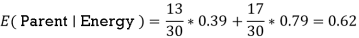
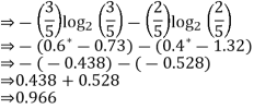
Now that we have the values of E(Parent) and E(Parent|Energy), we can calculate the information gain as follows:
Information gain = E (Parent) and E(parent|energy)
= 0.99 – 0.62
= 0.37
Our parent entropy was near 0.99, and based on this amount of information gain, we can estimate that if we make "Energy" our root node, the entropy of the dataset will fall by 0.37.
Similarly, we will calculate the knowledge gain for the other attribute "Motivation."
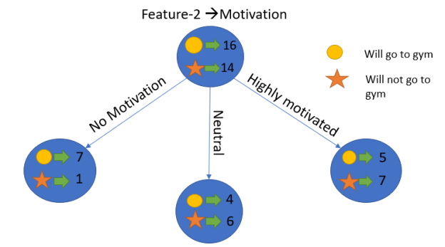
Let’s calculate the entropy here:
E(Parent) = 0.99


We'll do the following to see each node's weighted average entropy:

Now that we have the values of E(Parent) and E(Parent|Motivation), we can calculate the information gain as follows:
Information gain = E (Parent) and E(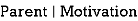 )
)
= 0.99 – 0.86
= 0.13
Greedy best-first search algorithm always selects the path which appears best at that moment. It is the combination of depth-first search and breadth-first search algorithms. It uses the heuristic function and search. Best-first search allows us to take the advantages of both algorithms. With the help of best-first search, at each step, we can choose the most promising node. In the best first search algorithm, we expand the node which is closest to the goal node and the closest cost is estimated by heuristic function, i.e.
f(n)= g(n).
Where, h(n)= estimated cost from node n to the goal.
The greedy best first algorithm is implemented by the priority queue.
Best first search algorithm:
Step 1: Place the starting node into the OPEN list.
Step 2: If the OPEN list is empty, Stop and return failure.
Step 3: Remove the node n, from the OPEN list which has the lowest value of h(n), and places it in the CLOSED list.
Step 4: Expand the node n, and generate the successors of node n.
Step 5: Check each successor of node n, and find whether any node is a goal node or not. If any successor node is goal node, then return success and terminate the search, else proceed to Step 6.
Step 6: For each successor node, algorithm checks for evaluation function f(n), and then check if the node has been in either OPEN or CLOSED list. If the node has not been in both list, then add it to the OPEN list.
Step 7: Return to Step 2.
Advantages:
- Best first search can switch between BFS and DFS by gaining the advantages of both the algorithms.
- This algorithm is more efficient than BFS and DFS algorithms.
Disadvantages:
- It can behave as an unguided depth-first search in the worst case scenario.
- It can get stuck in a loop as DFS.
- This algorithm is not optimal.
Example:
Consider the below search problem, and we will traverse it using greedy best-first search. At each iteration, each node is expanded using evaluation function f(n)=h(n) , which is given in the below table.
In this search example, we are using two lists which are OPEN and CLOSED Lists. Following are the iteration for traversing the above example.
Expand the nodes of S and put in the CLOSED list
Initialization: Open [A, B], Closed [S]
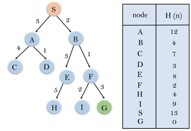
Iteration 1: Open [A], Closed [S, B]
Iteration 2: Open [E, F, A], Closed [S, B]
: Open [E, A], Closed [S, B, F]
Iteration 3: Open [I, G, E, A], Closed [S, B, F]
: Open [I, E, A], Closed [S, B, F, G]
Hence the final solution path will be: S----> B----->F----> G
Time Complexity: The worst case time complexity of Greedy best first search is O(bm).
Space Complexity: The worst case space complexity of Greedy best first search is O(bm). Where, m is the maximum depth of the search space.
Complete: Greedy best-first search is also incomplete, even if the given state space is finite.
Optimal: Greedy best first search algorithm is not optimal.
Key takeaway
Greedy best-first search algorithm always selects the path which appears best at that moment. It is the combination of depth-first search and breadth-first search algorithms.
Forward chaining is also known as forward deduction or forward reasoning when using an inference engine. Forward chaining is a method of reasoning that begins with atomic sentences in a knowledge base and uses inference rules to extract more information in the forward direction until a goal is reached.
Beginning with known facts, the Forward-chaining algorithm activates all rules with satisfied premises and adds their conclusion to the known facts. This procedure is repeated until the problem is resolved.
It's a method of inference that starts with sentences in the knowledge base and generates new conclusions that may then be utilized to construct subsequent inferences. It's a plan based on data. We start with known facts and organize or chain them to get to the query. The ponens modus operandi is used. It begins with the data that is already accessible and then uses inference rules to extract new data until the goal is achieved.
Example: To determine the color of Fritz, a pet who croaks and eats flies, for example. The Knowledge Base contains the following rules:
If X croaks and eats flies — → Then X is a frog.
If X sings — → Then X is a bird.
If X is a frog — → Then X is green.
If x is a bird — -> Then X is blue.
In the KB, croaks and eating insects are found. As a result, we arrive at rule 1, which has an antecedent that matches our facts. The KB is updated to reflect the outcome of rule 1, which is that X is a frog. The KB is reviewed again, and rule 3 is chosen because its antecedent (X is a frog) corresponds to our newly confirmed evidence. The new result is then recorded in the knowledge base (i.e. X is green). As a result, we were able to determine the pet's color based on the fact that it croaks and eats flies.
Properties of forward chaining
● It is a down-up approach since it moves from bottom to top.
● It is a process for reaching a conclusion based on existing facts or data by beginning at the beginning and working one's way to the end.
● Because it helps us to achieve our goal by exploiting current data, forward-chaining is also known as data-driven.
● The forward-chaining methodology is often used in expert systems, such as CLIPS, business, and production rule systems.
Backward chaining
Backward-chaining is also known as backward deduction or backward reasoning when using an inference engine. A backward chaining algorithm is a style of reasoning that starts with the goal and works backwards through rules to find facts that support it.
It's an inference approach that starts with the goal. We look for implication phrases that will help us reach a conclusion and justify its premises. It is an approach for proving theorems that is goal-oriented.
Example: Fritz, a pet that croaks and eats flies, needs his color determined. The Knowledge Base contains the following rules:
If X croaks and eats flies — → Then X is a frog.
If X sings — → Then X is a bird.
If X is a frog — → Then X is green.
If x is a bird — -> Then X is blue.
The third and fourth rules were chosen because they best fit our goal of determining the color of the pet. For example, X may be green or blue. Both the antecedents of the rules, X is a frog and X is a bird, are added to the target list. The first two rules were chosen because their implications correlate to the newly added goals, namely, X is a frog or X is a bird.
Because the antecedent (If X croaks and eats flies) is true/given, we can derive that Fritz is a frog. If it's a frog, Fritz is green, and if it's a bird, Fritz is blue, completing the goal of determining the pet's color.
Properties of backward chaining
● A top-down strategy is what it's called.
● Backward-chaining employs the modus ponens inference rule.
● In backward chaining, the goal is broken down into sub-goals or sub-goals to ensure that the facts are true.
● Because a list of objectives decides which rules are chosen and implemented, it's known as a goal-driven strategy.
● The backward-chaining approach is utilized in game theory, automated theorem proving tools, inference engines, proof assistants, and other AI applications.
● The backward-chaining method relied heavily on a depth-first search strategy for proof.
Key takeaway
Forward chaining is a type of reasoning that starts with atomic sentences in a knowledge base and uses inference rules to extract more material in the forward direction until a goal is attained.
The Forward-chaining algorithm begins with known facts, then activates all rules with satisfied premises and adds their conclusion to the known facts.
A backward chaining algorithm is a type of reasoning that begins with the objective and goes backward, chaining via rules to discover known facts that support it.
Bag of Words
Bag-of- Words is the most widely used natural language processing technique. This technique involves extracting words or features from a sentence, document, website, or other source and categorising them according to their frequency of occurrence. As a result, feature extraction is one of the most crucial aspects of the entire procedure.
Image Processing
One of the best and most interesting domains is image processing. In this area, you will essentially begin to interact with your photographs in order to comprehend them. To process a digital image or video, we employ a variety of approaches, including feature extraction and algorithms, to recognise features such as shapes, edges, and movements.
Auto-encoders
The primary goal of auto-encoders is to provide efficient data coding that is unsupervised. Unsupervised learning is the term used to describe this process. As a result, the feature extraction technique may be used to discover the essential features from the data to code by learning from the original data set's coding to create new ones.
References:
- Parag Kulkarni and Prachi Joshi, “Artificial Intelligence – Building Intelligent Systems”, PHI learning Pvt. Ltd., ISBN – 978-81-203-5046-5, 2015
- B Joshi, Machine Learning and Artificial Intelligence, Springer, 2020.
- Mohri, Rostamizdeh, Talwalkar, Foundations of Machine Learning, MIT Press, 2018.
- Artificial Intelligence by Elaine Rich, Kevin Knight and Nair, TMH


