Unit -5
Statistical quality control
5.1 Statistical concept
a) Systematic collection and recording of data accurately.
b) Analysing the data.
c) Practical implementation or Management action.
ADVANTAGES OF SQC
a) Efficiency and Cost reduction.
b) More effective pressure or control on quality efforts.
c) Reduction of scrap and Better utilization of raw material.
d) Improvement in inspection standards.
e) Easy detection of faults.
f) Reduction in consumer complaints and Improvement in producer-consumer relations.
g) Creating quality awareness amongst employees and Improvement in their morale.
h) Improves productivity.
i) Reduces wastage of men and machine hours.
j) Easy to apply.
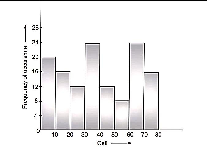
(a) Frequency Histogram
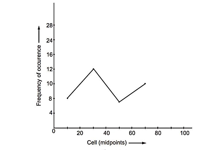
(b) Frequency Polygon
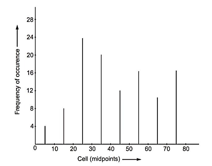
(c) Bar Chart
Attributes :-
Control Charts :-
Plotting of X̅ and R Chart
Step – I: Calculate Average ( X̅) and Range (R) for each sample.

x̿ = 
& 
where N = Number of samples
The control limits are given by,
Upper control limit X̅ = UCL X̅ = x̿ + 3σ X̅
Lower control limit X̅ = LCL X̅ = x̿ - 3σ X̅
Here, σ. X̅ = Standard deviation of averages = 
Where n = sample size
σ' = Standard deviation of universe = 
where, d2 is a factor depending upon sample size.
(i) UCL R = D4  and LCL R = D3
(ii) UCL R = D2 σ’ and LCL R = D1 σ’
(i) For X̅ chart, the central line on X̅ chart should be drawn as solid horizontal line as x̿. The upper and lower control limits should be drawn as dotted horizontal lines at the calculated values.
(ii) For R chart, central line on R chart should be drawn as solid horizontal line as  and control limits should be drawn as dotted horizontal lines.
The values of X̅1, X̅2, X̅3… X̅4 are plotted on X̅ chart, whereas, values of R1, R2, R3, … Rn are plotted on R chart. Points falling outside the control limits are indicated by cross, whereas, points falling inside the control limits are encircled.
Objectives of X̅ and R-chart
Limitations of X̅ and R-chart
Steps to Draw P-Chart
P = 
3. Compute  (Average fraction defective) as,
 =
= 
4. Compute control limits,
UCL P = 
LCL P = 
5. Plot each point as obtained and control limits as calculated. The points falling outside control limits are identified, (If any).
6. If the points fall outside the control limits, there may be two reasons:
(a) Assignable causes of variation may be present.
(b) Standard of Quality level is different for assumed standard P.
Objectives of P-Chart
Because of lower inspection and maintenance costs of P-chart, they usually have a greater area of economical applications than control charts used for variable.
“C” CHART
We have, Central line =  =
= 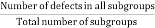
Upper control limit, UCL C = 
Lower control limit, UCL C = 
Applications of C Chart
(a) Number of surface defects in an aircraft wing.
(b) Number of defects such as blowholes, cracks in a casting.
(c) Number of imperfections observed in a cloth of unit area.
(d) Number of surface defects in galvanized sheet.
(e) Number of small holes in glass bottles.
Cp :-
• Process capability ratio or index is given by,
Cp = 
= 

Cpk :-
Cpk = min
Ppk :-
Ppk = min 
Advantages of PPAP
1. 100% inspection.
2. Sampling inspection or Acceptance sampling.
Advantages of Acceptance Sampling:
(i) The method is applicable in those industries where there is mass production and the industries follow a set production procedure.
(ii) The method is economical and easy to understand.
(iii) Causes less fatigue boredom.
(iv) Computation work involved is comparatively very small.
(v) The people involved in inspection can be easily imparted training.
(vi) Products of destructive nature during inspection can be easily inspected by sampling.
(vii) Due to quick inspection process, scheduling and delivery times are improved.
Limitations of Acceptance Sampling:
(i) It does not give 100% assurance for the confirmation of specifications so there is always some likelihood/risk of drawing wrong inference about the quality of the batch/lot.
(ii) Success of the system is dependent on, sampling randomness, quality characteristics to be tested, batch size and criteria of acceptance of lot.
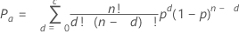
(a) N = Lot size, from which, samples are drawn.
(b) n = Sample size
(c) C = Acceptance number
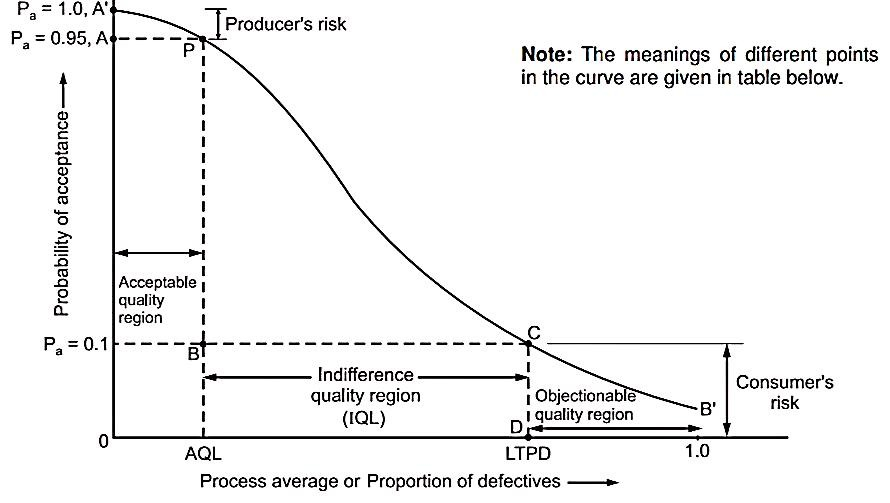
(a) Acceptance quality region.
(b) Indifference quality region
(c) Objectionable quality region.
AOQ = Pa · p’ 
where, Pa = Probability of acceptance
N = Lot size
n = Sample size
Characteristics of O.C. Curve
Significance of O.C. Curve
b. Stratified Sampling
c. Cluster Sampling
d. Sampling in Stages
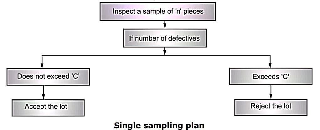
1. N = Lot size,
2. n = Sample size,
3. C = Acceptance number = Maximum number of allowable defectives in sample of size 'n'.
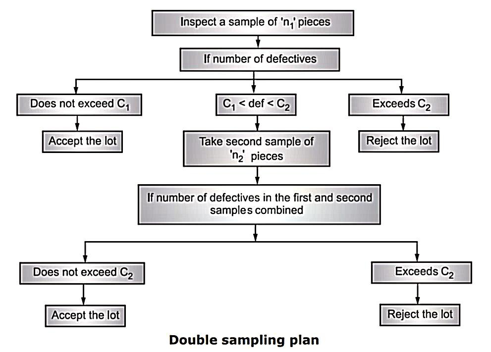
2. Double Sampling Plan
Let n1 = Number of pieces in the first sample.
C1 = Acceptance number for the first sample = Maximum number of defectives, that will permit the acceptance of lot on the basis of first sample
n2 = Number of pieces in the second sample.
n1 + n2 = Number of pieces in the two samples combined.
C2 = Acceptance number for the two samples combined = Maximum number of defectives, that will permit the acceptance of lot on the basis of first and second sample combined.
Advantages/Merits of Double Sampling Plan:
1. It gives second chance to the producer. Therefore, it is much preferred and acceptable to producers.
2. Cost of administration is moderate.
Disadvantages/Demerits:
1. Economical loss, if
(i) Samples do not represent the true picture of lot, and
(ii) Acceptance criteria (number) is not selected properly.
2. More record keeping is required, since decision is made on two samples drawn and number of parameters stated are more.
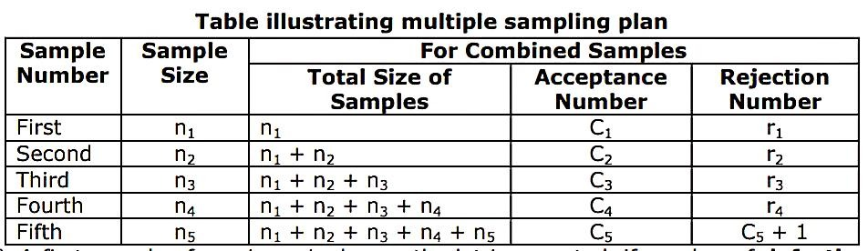
3. Multiple Sampling Plans
(i) A first sample of n1 pieces is drawn, the lot is accepted, if number of defectives are less than C1 and rejected, if more than r1.
(ii) But, if C1 < defectives < r1, a second sample of n2 pieces is drawn, the lot is accepted, if number of defectives are less than C2 in combined sample of ‘n1 + n2’ and rejected, if more than r2. The procedure is continued in accordance with the above table.
(iii) If by the end of fourth sample, the lot is neither accepted nor rejected, a sample of n5 pieces is drawn.
(iv) The lot is accepted, if the number of defectives in the combined sample of n1, n2, n3, n4, n5 is less than C5 and rejected, if more than C5 + 1.
Sr. No. | Feature | Single | Double | Multiple |
1 | Average number of | Generally large. | In between single and multiple. It is preferred to take second sample of size twice the size of first sample. | Low. |
2 | Acceptability to producer. | Poor, as it gives only one chance to decide, whether the lot is accepted or rejected | Most acceptable (Gives II nd chance). | Less acceptable, if indecision continues for a long period and more number of samples are drawn for making decision. |
3 | Cost of Administration | Lowest. | In between. | Largest. |
4 | Information available about prevailing quality level. | Largest. | In between. | Lowest. |
5 | Number of samples | One | Two | Multiple. |
6 | Variability of inspection load [i.e. number of items undergoing inspection] | Constant | Variable, depending upon behaviour of first sample. | Highly variable. |
7 | Estimation about quality of a lot | Best | Intermediate | Difficult to estimate. |
8 | Decision of 'Acceptance' or 'Rejection' is based on | One sample | Two samples combined. | Multiple samples combined. |
n = n'p/ P
Where n'p = Total number of defectives.
P = % defectives in a lot
AOQ = Pa · p’ 
where, Pa = Probability of acceptance
N = Lot size
n = Sample size
c = acceptance number
n = sample size
p = fraction defective
Numerical


Solution
Given
n = 4
N = 20
 = 825.60
 = 5.60 mm
Specification limit = 41.0  0.40 mm
d2 = 2.059
x̿ =  =
=  = 41.28
 =
=  = 0.28
 = 0.1359
 =
= 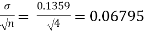
Upper control limit X̅ = UCL X̅ = x̿ + 3σ X̅ = 41.28 + 3 x 0.06795 = 41.4838
Lower control limit X̅ = LCL X̅ = x̿ - 3σ X̅ = 41.28 - 3 x 0.06795 = 41.0761
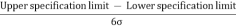
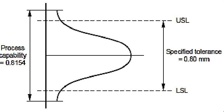
Process capability 6  = 6 x 0.1359 = 0.8154
Upper control limit USL = 41 + 0.4 = 41.4 mm
Lower control limit LSL = 41 – 0.4 = 40.6 mm
Specified tolerance = USL – LSL = 41.4 – 40.6 = 0.8 mm
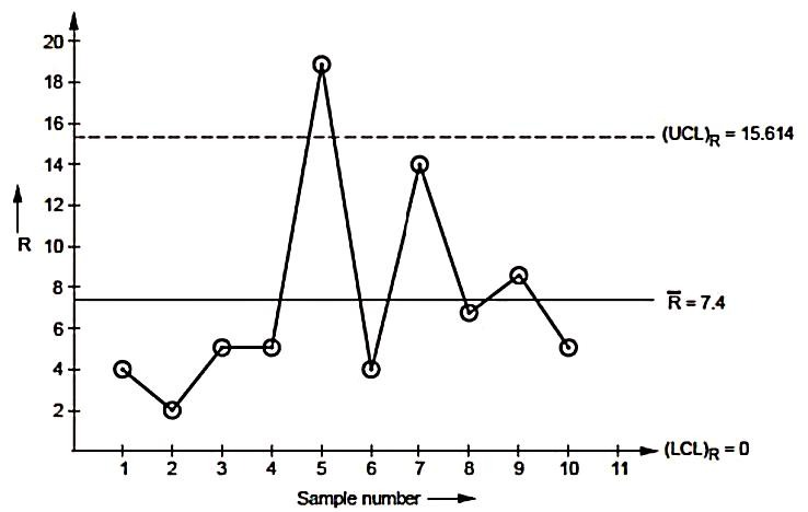
2. Following data shows value of sample mean  & range R for 10 samples of size 5 each. Calculate control limits for mean & range chart. Determine Whether the process is under control or not.
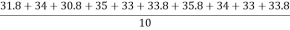
Sample no. | X̅ | R |
1 | 31.8 | 4 |
2 | 34 | 2 |
3 | 30.8 | 5 |
4 | 35 | 5 |
5 | 33 | 19 |
6 | 33.8 | 4 |
7 | 35.8 | 14 |
8 | 34 | 7 |
9 | 33 | 9 |
10 | 33.8 | 5 |
Component specification limits 40.37  1
1
Take A2 = 0.577, D3 = 0, D4 = 2.110
Solution
Given
Specification limits 40.37  1
1
A2 = 0.577,
D3 = 0,
D4 = 2.110
N = 20
n = 5
x̿ =  =
=  = 33.5
 =
=  = 7.4
= 7.4
 x̿ + A2
 = 33.5 + 0.577 x 7.4 = 37.7698
 x̿ - A2
 = 33.5 - 0.577 x 7.4 = 29.2302
 D4 = 7.4 x 2.110 = 15.614
 D3 = 7.4 x 0 = 0
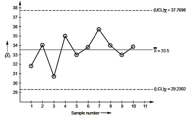
 x̿ + 3σ X̅
37.7698 = 33.5 + 3σ X̅
σ X̅ = 1.4232
 =
= 
1.4232 x  = 3.1823
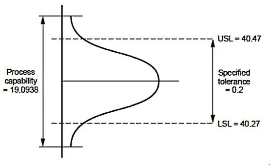
Process capability 6  = 6 x 3.1823 = 19.0938
Upper control limit USL = 40.37 + 0.1 = 40.47 mm
Lower control limit LSL = 40.37 – 0.1 = 40.27 mm
Specified tolerance = USL – LSL = 40.47 – 40.27 = 0.2 mm
3. Following is the record for successive lots of a part being produced by a plastic moulding process. As each lot is come off the line a random sample of 150 pieces were inspected ( results are expressed to the nearest 0.1 %) calculate  control limits & plot control chart & comment.
Lot no | Sample size | Number of defectives |
1 | 150 | 4 |
2 | 150 | 8 |
3 | 150 | 2 |
4 | 150 | 4 |
5 | 150 | 4 |
6 | 150 | 6 |
7 | 150 | 10 |
8 | 150 | 4 |
9 | 150 | 6 |
10 | 150 | 4 |
Solution
Given
n = 150
 =
=  =
= 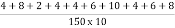 = 0.03733
UCL P =  = 0.03733 +3
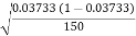 = 0.08376
LCL P =  = 0.03733 - 3
 = 0.00910
Fraction defectives = 
Lot no | Number of defectives | Fraction defectives |
1 | 4 | 0.026 |
2 | 8 | 0.053 |
3 | 2 | 0.013 |
4 | 4 | 0.026 |
5 | 4 | 0.026 |
6 | 6 | 0.04 |
7 | 10 | 0.06 |
8 | 4 | 0.026 |
9 | 6 | 0.04 |
10 | 4 | 0.053 |
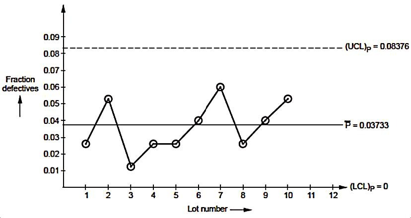
From the above graph it is observed that, all the lots fall inside the control limit which makes the process in control.
4. Following given table shows the number of defectives found in inspection of 9 lot of 100 items each.
Lot no | Number of defectives |
1 | 6 |
2 | 3 |
3 | 1 |
4 | 4 |
5 | 3 |
6 | 11 |
7 | 5 |
8 | 2 |
9 | 3 |
Determined the controlled limit for fraction defective chart. State whether the process is in control. If not by eliminating outside control limit point, what will be the new control limit ?
Solution
Given
n = 100
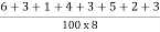
Number of lot = 9
 =
=  =
= 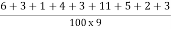 = 0.0422
UCL P =  = 0.0422 +3
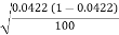 = 0.1025
LCL P =  = 0.0422 - 3
 = -0.01811
Fraction defectives = 
Lot no | Number of defectives | Fraction defectives |
1 | 6 | 0.06 |
2 | 3 | 0.03 |
3 | 1 | 0.01 |
4 | 4 | 0.04 |
5 | 3 | 0.03 |
6 | 11 | 0.11 |
7 | 5 | 0.05 |
8 | 2 | 0.02 |
9 | 3 | 0.03 |
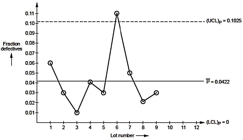
From the above graph it is observed that, the lot number 6 falls outside the control limit which makes the process out of control.
As lot number 6 makes the process out of control, eliminate lot number 6
 =
=  =
=  = 0.03375
New UCL P =  = 0.03375 +3
 = 0.08792
New LCL P = 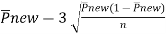 = 0.03375 - 3
 = -0.02042
5. Calculate AOQ for single sampling plan using following data
Solution
Given
N = 10000
c = 1
P = 0.5% = 0.005
Pa = 0.525
n'p = 1.5
n = n'p/ P = 1.5/0.005 = 300 units
AOQ = P x Pa = 0.005 x 0.525 = 0.002625 = 0.2625 %
If defectives are to be replaced then
AOQ =  P x Pa =
  x 0.005 x 0.525 = 0.00254 = 0.254 %
Reference:


