Unit 1
Signals and Spectra
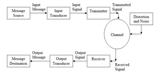
Figure 1. Block Diagram of Communication system
- Message Source: The originator of the message
- Input Message: The message/data/info that is to be communicated
- Input Transducer: Converts the input message into electrical form
- Input Signal: The data in electrical form (this is a baseband signal)
- Transmitter: Modifies the signal for transmission
- Channel: The medium over which the transmitted signal is sent (e.g., wire, air, optical fibre, free space)
- Distortion/Noise: External signals/features that affect the signal
- Receiver: Modifies the received signal, undoing the modifications done by the transmitter
- Output Transducer: Converts message from electrical signal back into its original form
- Output Message: The message/data/info that has been communicated
- Message Destination: Who/what the message/data/info was intended for.
Key Takeaways:
- Communication system
- Components of Communication system
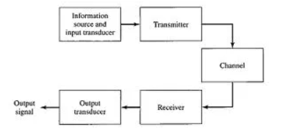
Figure 2. Analog communication
In Analog Communication, the message, or the information which has to be transmitted is analog in nature. This analog message is obtained from the source such as speech, video, audio etc.
The message signal in this case are modulated at high carrier frequency inside the transmitter to produce modulated signal. This modulated signal is then transmitted with the help of transmitting antenna to travel across the transmission channel.
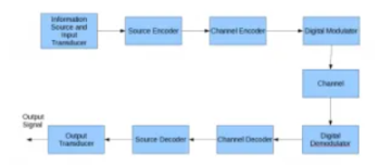
Figure 3.Digital Communication
In digital communication the purpose of these systems is to message or sequence of symbols that are coming out from the source to the destination point at a very high data rate and accuracy as possible. The source and destination points are physically separated in the space and a communication channel is used to connect the source and the destination.
Key Takeaways:
- Analog signal and its importance
- Digital signal and its importance
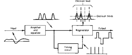
Figure 4. Block diagram of Regenrative Repeaters
The regenerative repeater and shows typical waveforms corresponding to each functional stage of signal processing.
At the first stage of signal processing is amplification and equalization. With many regenerative repeaters, equalization is a two-step process.
The first is a fixed equalizer that compensates for the attenuation-frequency characteristic caused by the standard length of transmission line between repeaters which is often 6000 ft or 1830 m.
The second equalizer is variable and compensates for departures between nominal repeater section length and the actual length as well as loss variations due to temperature.
The adjustable equalizer uses automatic line build-out (ALBO) networks that are automatically adjusted according to characteristics of the received signal.
The signal output of the repeater must be precisely timed to maintain accurate pulse width and space between the pulses. The timing is derived from the incoming bit stream.
The incoming signal is rectified and clipped, producing square waves that are applied to the timing extractor, which is a circuit tuned to the timing frequency. The output of the circuit controls a clock-pulse generator that produces an output of narrow pulses that are alternately positive and negative at the zero crossings of the square-wave input.
The narrow positive clock pulses gate the incoming pulses of the regenerator, and the negative pulses are used to run off the regenerator. Thus, the combination is used to control the width of the regenerated pulses.
Key Takeaways:
- Regenerative repeater and its importance
- Block diagram of regenerative repeater
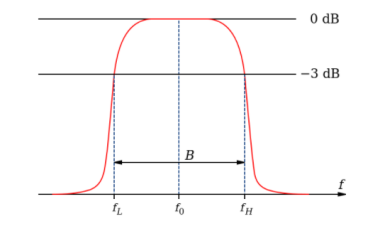
Figure 5. Signal Bandwidth
The bandwidth of a signal is defined as the difference between the upper and lower frequencies of a signal generated. Bandwidth (B) of the signal is equal to the difference between the higher or upper-frequency (fH) and the lower frequency (fL). It is measured in terms of Hertz (Hz) i.e. the unit of frequency.
Power is defined as the amount of energy consumed per unit time. This quantity is useful if the energy of the signal goes to infinity or the signal is “not-squarely-summable”. For “non-squarely-summable” signals, the power calculated by taking the snapshot of the signal over a specific interval of time as follows
1) Take a snapshot of the signal over some finite time duration
2) Compute the energy of the signal Ex
3) Divide the energy by number of samples taken for computation N
4) Extend the limit of number of samples to infinity N -> ∞. This gives the total power of the signal.
In discrete domain, the total power of the signal is given by
Px = lim N-> ∞ 1/ 2N +1  2
2
From these equations, different forms of the same computation are found. The only difference is the number of samples taken for computation. The denominator changes according to the number of samples taken for computation.
Px = lim N-> ∞ 1/2N 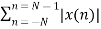 2
2
Px = lim N-> ∞ 1/N 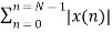 2
2
Px = lim N-> ∞ 1/N1-No+1  2
2
Find the power of the signal
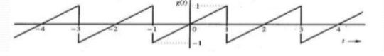
Pg = ½  2(t) dt = ½
  2 dt = 1/3
The signal power is square pf its rms value. Therefore, the rms value of the signal is 1/√3
Key Takeaways:
- Signal Bandwidth
- Power of signal and its derivation
The term “size of a signal” is used to represent “strength of the signal”. It is crucial to know the “size” of a signal used in a certain application.
For example, if we want to know the amount of electricity needed to power LCD monitor as opposed to CRT monitor. Both of these applications are different and have different tolerances. Thus, the amount of electricity driving these devices will also be different.
Signals are classified into the following categories:
- Continuous Time and Discrete Time Signals
- Deterministic and Non-deterministic Signals
- Even and Odd Signals
- Periodic and Aperiodic Signals
- Energy and Power Signals
- Real and Imaginary Signals
Continuous Time and Discrete Time Signals
A signal is said to be continuous when it is defined for all instants of time.

Figure 6. Continuous signal
A signal is said to be discrete when it is defined at only discrete instants of time

Figure 7. Discrete signal
Deterministic and Non-deterministic Signals
A signal is said to be deterministic if there is no uncertainty with respect to its value at any instant of time or the signals which can be defined exactly by a mathematical formula are known as deterministic signals.

Figure 8. Deterministic Signal
A signal is said to be non-deterministic if there is uncertainty with respect to its value at some instant of time. Non-deterministic signals are random in nature hence they are called random signals. Random signals cannot be described by a mathematical equation. They are modelled in probabilistic terms.

Figure9. Non- deterministic signal
Even and Odd Signals
A signal is said to be even when it satisfies the condition x(t) = x(-t)
Example 1: t2, t4… cost etc.
Let x(t) = t2
x(-t) = (-t)2 = t2 = x(t)
∴, t2 is even function
Example 2: As shown in the following diagram, rectangle function x(t) = x(-t) so it is also even function.

A signal is said to be odd when it satisfies the condition x(t) = -x(-t)
Example: t, t3 ... And sin t
Let x(t) = sin t
x(-t) = sin(-t) = -sin t = -x(t)
∴, sin t is odd function.
Any function ƒ(t) can be expressed as the sum of its even function ƒe(t) and odd function ƒo(t).
ƒ(t ) = ƒe(t ) + ƒ0(t )
Where
ƒe(t ) = ½[ƒ(t ) +ƒ(-t )]
Periodic and Aperiodic Signals
A signal is said to be periodic if it satisfies the condition
x(t) = x(t + T) or x(n) = x(n + N).
Where
T = fundamental time period,
1/T = f = fundamental frequency.

Figure 10. Periodic signal
The above signal will repeat for every time interval T0 hence it is periodic with period T0.
Energy and Power Signals
A signal is said to be energy signal when it has finite energy.
Energy E =  2 (t) dt
A signal is said to be power signal when it has infinite power.
Power P = lim T->∞ 1/2T  2 (t) dt
NOTE: A signal cannot be both, energy and power simultaneously. Also, a signal may be neither energy nor power signal.
Power of energy signal = 0
Energy of power signal = ∞
Real and Imaginary Signals
A signal is said to be real when it satisfies the condition x(t) = x*(t)
A signal is said to be odd when it satisfies the condition x(t) = -x*(t)
Example:
If x(t)= 3 then x*(t)=3*=3 here x(t) is a real signal.
If x(t)= 3j then x*(t)=3j* = -3j = -x(t) hence x(t) is a odd signal.
Note: For a real signal, imaginary part should be zero. Similarly, for an imaginary signal, real part should be zero.
Key Takeaways:
- Size of signal
- Classification of signal
Exponential Fourier series
The exponential Fourier series is another form of Fourier series. Using Euler’s identity, we can write
An cos(Ω0nt +  n ) = An [ ej(Ω0nt +
  n) –e -j(Ω0nt +
  n)]
n)]
2
x(t) = A0 +  ej(Ω0nt +
  n) –e- j(Ω0nt +
  n)]
n)]
= A0 +  e j(Ωont) ejƟn – e - j(Ωont) e j(-Ɵn)
= A0 +  ej
ej n ) ej(Ω0nt ) + (An/2 e-j
  n ) e- j(Ω0t ) ] -------- (1)
Let n=-k
x(t) = A0 +  ejƟn ) ej(Ω0nt ] +
  e j Ɵk ) e j(Ω0kt ) ------- (2)
Comparing (1) and (2) we get
An = Ak (- n ) =
n ) =  k n>0 k<0-------------------(3)
Let us define c0 = A0; cn =An/2 ej Ɵn for n>0
By changing the index from k to n and combining into one equation we get
x(t) = A0 +  e j ) ej(Ω0nt) +
  ej
ej n) ej(Ω0nt)]
x(t) =  n ej(Ω0nt)]
The above series is known as Exponential Fourier Series.
To develop the coefficients of the the exponential Fourier series
We know that
x(t) =  n ej(Ω0nt)] where Ω0 = 2π/T
Multiply e-jk Ω0 t and integrate over one period. Then
 e-jk Ω0 t dt =
 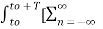 cn ej(Ω0nt) ] e-jk Ω0 t dt
=  cn
cn  ej(Ω0nt) e-jk Ω0 t dt
Substituting the relation  e-jk Ω0 t dt = 0 for k ≠n and T when k=n
 e-jk Ω0 t dt = T ck
Therefore
Ck = 1/T  e-jk Ω0 t dt
Or
Cn = 1/T  e-jk Ω0 t dt
Where Cn are the Fourier series coefficients of exponential Fourier series.
Compute the Fourier series f(t) where f(t) is the square wave with period 2π which is defined over one period by
f(t) = { -1 for -π  t
t
1 for 0 <π
<π
f(t) = ao/2 +  cos(nt) + bn sin(nt))
Where
Ao =1/π  dt an = 1/π
  cos nt dt bn =1/π
  cos nt dt
By applying these formulas to the above wave form we have to split the integrals into two pieces corresponding to where f(t) is +1 and where it is -1.
Thus for n 0; an = -sin (nt)/nπ| 0 -π + sin(nt) /n
 | π 0 =0
For n=0 ao = 1/π  dt =0
dt =0
Likewise
Bn = 1/π sin(nt) dt = 1/ π
  sin(nt) dt + / π
  sin(nt) dt
= cos(nt)/nπ | -π 0 - cos(nt)/nπ| π 0 = 1 – cos(-nπ)/nπ - cos(nπ)-1/nπ
= 2/nπ (1-cos(nπ) ) = 2/nπ( 1 – (-1) n) = { 4/nπ for n odd
0 for n even
This then gives the Fourier series for f(t)
f(t) =  sin(nt) = 4/π ( sint + 1/3 sin(3t) + 1/5 sin(5t)
+………………………………….
Key Takeaways:
- Exponential Fourier Series definition
- Derivation of Exponential Fourier series
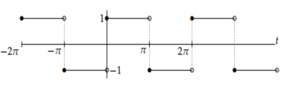
The Fourier transform doesn't break up a signal into sinusoids, it breaks it up into complex exponentials called as "complex sinusoids".
F(w) =  e -jwt dt ---------------------------------------------------(1)
These are actually spirals, spinning around in the complex plane:
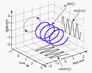
Figure 11. Negative frequencies
Spirals can be either left-handed or right-handed that is rotating clockwise or counter- clockwise, which is where the concept of negative frequency comes from.
In the case of real signals, there are always two equal-amplitude complex exponentials, rotating in opposite directions, so that their real parts combine, and imaginary parts cancel out, leaving only a real sinusoid as the result.
This is why the spectrum of a sine wave always has 2 spikes, one positive frequency and one negative. Depending on the phase of the two spirals, they could cancel out, leaving a purely real sine wave, or a real cosine wave, or a purely imaginary sine wave, etc.
The negative and positive frequency components are both necessary to produce the real signal, but the other side of the spectrum doesn't provide any extra information, so it's often hand-waved and ignored.
For the general case of complex signals, you need to know both sides of the frequency spectrum.
Consider the Fourier transform pair of a complex sinusoid
e jwot 
 + wo)
+ wo)
For a pure sinusoid (real) we have Euler’s relation
Cos(wot) = e jwot + e-jwot / 2
And hence, its Fourier transform pair
Cos(wot)  δ(w+wo) + δ(w-wo)
It has two frequencies: a positive one at ω0 and a negative one at −ω0 .
The complex sinusoid of aeȷω0t is widely used because it is incredibly useful in simplifying our mathematical calculations. However, it has only one frequency and a real sinusoid actually has two.
Negative frequencies are used all the time when doing signal or system analysis.
Key Takeaways:
- Concept of negative frequencies
- Importance of negative frequencies
The Fourier Transform is a mathematical technique that transforms a function of time, x(t), to a function of frequency, X(ω).
The Fourier Transform of a function can be derived as a special case of the Fourier Series when the period, T→∞
x(t) =  e jnwot ……………………………………………….(1)
Where cn is given by the Fourier series analysis equation
Cn = 1/T  e -jnwot dt
Which can be rewritten as
Tcn =  e -jnwot dt
As T→∞ the fundamental frequency wo=2π/T becomes extremely small and the quantity now becomes continuous quantity that can take on any value so we define w=now . Also X(w) = Tcn .
X(w) =  e-jwt dt
The Inverse Fourier transform
x(t) =  ejnwot
  ejnwot . 1/T
Properties
(i) Linearity
If x(t)  X(jw)
X(jw)
y(t)  Y(jw)
Y(jw)
Then
a x(t) + b y(t)  a X(jw) + b Y(jw)
(ii) Time shifting
If x(t)  X(jw)
X(jw)
Then
x(t-to)  e -jwto X(jw)
Find the Fourier transform of the signal as shown in figure
This signal can be obtained as a linear combination of
x(t) = ½ x1(t-2.5) + x2(t-2.5)
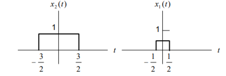
Where x1(t) and x2(t) are rectangular pulse signals and their Fourier transforms are
X1(jw) = 2 sin (w/2) / w and X2(jw) = 2 sin (3w/2)/w
Using linearity and time shifting properties of Fourier transform yields
X(jw) = e -j5w/2 { sin(w/2) + 2 sin(3w/2) /w}
Conjugate Property:
If x(t)  X(jw)
X(jw)
Then
x* (t)  X *(-jw)
Differentiation and Integration
If x(t)  X(jw)
X(jw)
Then
Dx(t)/dt  jw X(jw)
 dτ
dτ 1/jw X(jw) + π X(0) δ(w)
Consider the Fourier transform of the unit step x(t) = u(t).
We know that
g(t) =  1
1
Also note that
x(t) =  ) dτ
) dτ
The fourier transform of this function is
X(jw) = 1/jw + π G(0) δ(w) = 1/jw + π δ(w)
Where G(0) =1 .
Find the Fourier transform of the function x(t) as shown in figure.
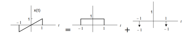
From the above figure we see that g(t) = d x(t) /dt is a sum of rectangular pulse and two impulses.
G(jw) = (2 sin w/w) – e jw – e -jw
Using integration property we obtain
X(jw) = G(jw) / jw + π G(0) δ(w) = 2 sin w/ j w 2 – 2 cos w / jw
It can be found that X(jw) is purely imaginary and odd which is consistent with the fact that x(t) is real and odd.
Time and Frequency scaling
If x(t)  X(jw)
X(jw)
Then
x(at) = 1/ |a| X(jw/a)
Parseval’s relation
If x(t)  X(jw)
X(jw)
We have
 x(t)| 2 dt = 1/ 2 π
  X(jw)| 2 dw
Parseval’s relation states that the total energy may be determined either by computing the energy per unit time |x(t)| 2 and integrating over all the time by computing the energy per unit frequency |X(jw)| 2 / 2 π and integrating over all frequencies.
For this reason |X(jw)| is often referred to as energy-density spectrum.
Convolution properties
y(t) = h(t) * x(t)  Y(jw) = H(jw) X(jw)
Multiplication property
r(t) = s(t) p(t)  δ R(jw) = 1/2π
  (j
(j ) P(j(w-
 ) d
) d
Multiplication of one signal by another can be thought as one signal to scale or modulate the amplitude of the other consequently the multiplication of two signals is referred to as amplitude modulation
Key Takeaways:
- Defintion of Fourier transform
- Properties of Fourier transform
Spectrum shifting (technically called "single sideband modulation") can be done with two sinewave oscillators that are in quadrature (90 degrees out of phase), a phase-shifting allpass filter that shifts all frequencies 90 degrees with respect to the input, and a couple of ringmodulators. The ringmodulators multiply the two phaseshifted signals with the two sinewaves. The outputs of the ringmodulators are then summed. The effect is that all frequencies (=harmonics) are shifted up or down by a fixed number of Hz, this number being the frequency of the two sinewaves. This means that the stronger the effect the more the harmonics lose their harmonic relation. . A shift of a few Hz can e.g. Make a static synthetic sound more lively. The difficulty in constructing such a frequency shifter is to make the phase-shifting filter (usually called a "Hilbert Transformer"). Such a filter usually only gives the desired phase-shifting properties over a limited frequency range.
Key Takeaways:
- Frequnecy shifting
- Importance of frequency shifting
A baseband signal can be transmitted over a pair of wires as in a telephone, co-axial cables, or optical fibres.
But a baseband signal cannot be transmitted over a radio link or a satellite because this would require a large antenna to radiate the low-frequency spectrum of the signal.
Hence the baseband signal spectrum must be shifted to a higher frequency by modulating a carrier with the baseband signal. This can be done by amplitude and by angle modulation (frequency and phase).
A bandpass signal is a signal containing a band of frequencies not adjacent to zero frequency, such as a signal that comes out of a bandpass filter.
Figure 12. Base band and Band pass signals
Key Takeaways:
- Concept of base band signal
- Concept of band pass signal
If 𝑥(𝑡) and 𝑦(𝑡) are input and output of a LTI system with impulse response ℎ(𝑡), then:
𝑌(𝜔) = 𝐻 𝜔 𝑋(𝜔)
• We can, therefore, perform LTI system analysis with Fourier transform in a way similar to that of Laplace transform.
• However, FT is more restrictive than Laplace transform because the system must be stable and 𝑥(𝑡) must itself be Fourier transformable.
• Laplace transform can be used to analyse stable and unstable systems, and applies to signals that grow exponentially.
• If a system is stable, it can be shown that the frequency response of the system 𝐻(𝑗𝜔) is just the Fourier transform of ℎ(𝑡) (i.e., 𝐻(𝜔)): 𝐻 𝜔 = 𝐻(𝑠)| 𝑠=𝑗w
The defining properties of any LTI system are linearity and time invariance.
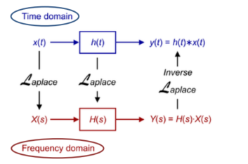
Figure 13. Signal transmission LTI
By steady state we mean a sinusoidal excitation.
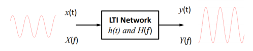
Figure 14. Sinusodial excitation
A sinusoidal signal of frequency f at the input, x(t), produces a sinusoidal signal of frequency f at the output, y(t). The output y(t) Is given by x(t) y(t) H(f) will modify input x(f) by a change in magnitude and phase.
Key Takeaways:
- LTI system
- Signal transmission through LTI system
- Means of signal transmission
The signal energy in the signal x(t) is
E =  x(t)| 2 dt
If 0< E< ∞, then the signal x(t) is called an energy signal.
Let us consider a periodic signal (tx ) with period . The signal energy in one period is
E1 =  2 dt
2 dt
And energy in n period is
En = nE1= n  2 dt
2 dt
Energy spectral density
Let f(t) be an electric potential in volt applied across a resistance R=1 ohm. The total energy in such a resistance is given by
E =  f 2 (t) /R} dt -------------------------------------------(1)
Since the resistance value is unity the dissipated energy is known as normalized energy.
Parsevals theorem states that if a function f(t) is generally complex and if F(jw) is Fourier transform of f(t) then
 f 2 (t) /R} dt = 1/2π
  2 dw
2 dw
The function |F(jw)| 2 is called the energy spectral density or simple energy density of f(t).
Key Takeaways:
- Signal Energy
- Energy spectral density
The signal power in the signal x(t) is
P = lim T->∞ 1/2T  2 dt
2 dt
If 0< E< ∞, then the signal x(t) is called an energy signal. However, there are signals where this condition is not satisfied. For such signals we consider power.
If 0< P< ∞, then the signal is called a power signal.
Power spectral density
For a real power signal f(t) the power spectral density is denoted by Sff(w) is by definiton the Fourier trnsform of autocorrelation function
Sff(w) = F{rff(t0} = Rff(jw)
Since rff(t) is real and even its transform Sff(w) is real and even. We have
Sff(w) = 2  cos wt dt
And rff(t)= 1/π  cos wt dw
Let fT(t) = f(t) π T(t) = f(t) { u(t+T) – u(t-T)}
Where fT(t) is a truncation of f(t).
We have
ST(w) = 1/2T |FT(jw)|2
It can be shown that Sff(w)is the limit as T tends to infinity of ST(w)
Sff(w) = lim T-> ∞ ST(w)= lim T->∞ 1/2T |FT(jw)| 2
In fact
Sff(w) = F{rff(t)} F{ lim T-> ∞ 1/2T  fT(
fT( dτ
dτ
= lim T-> ∞ 1/2T  fT(
fT( dτ
dτ
= lim T-> ∞ 1/2T  fT(
fT( dτ e -jwt dt
= lim T-> ∞ 1/2T  e -jwt dt
Let
t + τ = x
Sff(w) = lim T->∞ 1/2T  T (τ) d
 T (x) e -jw(x-τ) dx dτ
= lim T->∞  T (τ) e jwτ dτ
= lim T->∞ 1/2T FT(jw)  T (τ) e jwτ dτ = lim T->
  1/2T FT(jw)
= lim T->∞ 1/2T |FT(jw)| 2  = lim T->∞ ST(w)
Key Take Aways:
- Signal Power
- Power Spectral Density
If g(t) and y(t) are input and the corresponsing output of LTI system then
Y(w) = H(w) G(w)
Therefore |Y(w)| 2 = |H(w) | 2 |G(w)| 2
The time autocorrelation function Rg(τ) of real deterministic power signal g(t) is defined as
Rg(τ) = lim T-> ∞ 1/T  g(t+τ) dt
We have that
R g(τ)  Sg(w)
Sg(w)
If g(t) and y(t) are input and the corresponding output of LTI system then
Sy(w) = |H(w)| 2 Sg(w)
Thus the output signal PSD is |H(w)| 2 the input signal PSD.
Key Takeaways:
- Input signal PSD
- Output signal PSD
- Relation of output and input.
Consider
u(t) =  p(t-nT)
Where u(t) is cyclostationary wrt T if {bn } is stationary
u(t) is wide sense cyclostationary wrt to T if {bn} is WSS
Suppose Rb[k] = E[bnbn-k]
Let Sb(z) =  z-k
z-k
The PSD of u(t) is given by
Su(f) = Sb ( e j2πfT ) | P(f)|2 /T
Ru( τ) = 1/T  (t+
(t+ dt
dt
= 1/T  [ bn bm p(t-nT + τ) p*(t-mT)] dt
= 1/T  [ bn bm*p(t-nT+τ) p*(t-mT)] dt
= 1/T  [ bm+k bm * p(λ -kT + τ) p*(λ)] dλ
= 1/T 
 (λ -kT +τ) p*(λ) dλ
Ru(τ) = 1/T  b[k]
b[k]  λ – kT + τ) p*(λ) dλ
=  λ + τ) p*(λ) dλ = | P(f) | 2
=  λ -kT +τ) p*(λ) dλ = |P(f) 2 |e -j2πfkT
= Sb ( ej2πfT) |P(f)|2/T
Where Sb(z) =  [k] z -k
Key Takeaways:
- PSD of modulated signal
- Derivation of PSD
References:
Digital Communication Systems Book by Simon S. Haykin
Principles of digital communication Textbook by Robert G. Gallager
Digital Communications Book by John G Proakis and Masoud Salehi
Digital Communications Book by Sanjay Sharma
Digital Communication Book by J.S. Chitode


