Unit – 3
Numerical Methods
Example 1:
Newton Forward differences 
Y( + rh) =
 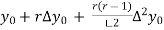 +
+ 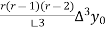 + ….
+ ….
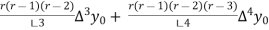
Newton Backward difference 
Y(x) = y ( ) =
) =  +
+  +
+ 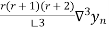 + …….
+ …….
 The population of a city in the decimal census is given in the following table
Year X | 1891 | 1901 | 1911 | 1921 | 1931 |
Population Y (in thousand) | 46 | 66 | 81 | 93 | 101 |
Approximate the population of the city in the years 1895 and 1925
Ans  Difference Table
X | Y |
|
|
|
|
1891 | 46 | 20 |
|
|
|
1901 | 66 | 15 | -5 | -2 |
|
1911 | 81 | 12 | -3 | -1 | -3 |
1921 | 93 | 8 | -4 |
|
|
1931 | 101 |
|
|
|
|


Compute the population in 1895
Using Newton forward differences formula
Y(x) =  +
+  +
+  + …
+ …
Let  = 1891 h = 10 X =
  = 1895
r = 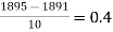
y(1895) = 46 + 0.4(20)+  (-5)+
(-5)+ 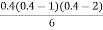 (2) +
(2) + 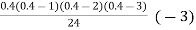
= 54.85 thousand (Approx)
Compute the population in 1925 using backward difference formula
Y(x) =  + r
+ r + ……..
Let  = 1931 r =
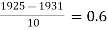
Y(1925) = 101 + (0.6) 8 +  +
+ 
= 96.84 thousand only.
 Interpolation with unequal intervals
Newton divided difference formula 
f( ) =
) = 
f( ) =
) = 
 (x) = f(
 ) + (x -
  )f(
)f( ) + (x -
 )(x -
)(x -  )f(
)f( ) + ……
e.g using divided difference interpolation Find f(x)
x | 0 | 1 | 2 | 4 | 5 | 6 |
Y = f(x) | 1 | 14 | 15 | 5 | 6 | 19 |
 The divided difference table
x | 4 | d.d of order1 | d.d of order2 | d.d of order3 | d.d of order4 | d.d of order5 |
0 | 1 |
|
|
|
|
|
1 | 14 | 13 | -6 | 1 |
|
|
2 | 15 | 1 | -2 | 1 | 0 |
|
3 | 5 | -5 | 2 | 1 | 0 | 0 |
4 | 6 | 1 | 6 |
|
|
|
5 |
| 13 |
|
|
|
|
6 | 19 |
|
|
|
|
|
Using formula
Y = f(x)=  + (x -
  )
) + (x -
  ) (x-
) (x-  )f
)f + (x -
  )(x -
)(x -  )(x -
)(x -  ) f
) f +…….
+…….
= 1 + (x - 0)(13) + (x - 0)(x-1)(-6)+ (x - 0)(x-1)(x -2)(1) + (x -0)(x-1)(x - 2)(x - 4)(0) + (x -0)(x - 1)(x -1) (x - 2)(x - 4)(x -5)0+ 0
= 1 + 13x + ( - x)(-6)+ (
 + 2x)(1) + 0
= 1 + 21x - 9
f(x) = 
 Using Lagranye’s interpolation Solve the following data
x | 300 | 304 | 305 | 307 |
| 2.477 | 2.482 | 2.484 | 2.487 |

Calculate the approximate value of 
Ans. Using formula
y =  =
=  +
+ 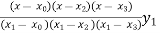 +
+ 
= 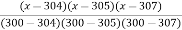 (2.477) +
 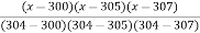 (2.482) +
 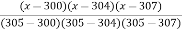 (2.484) +
 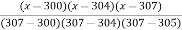 (2.4871)
 =
=  (2.477) +
 (2.4829) +
  (2.4843) +
  (2.4871)
= 1.2739 + 4.9658 – 4.4717 + 0.7106
= 2.4786
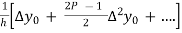
Newton forward difference formula
Y =  + P
+ P +
+  +
+ 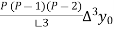 + ….
+ ….
 =
= 
 =
= 
( =
= 
Where h = 
 =
= 
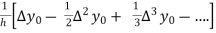
Backward difference 
 =
= 
(  =
= 
(1) Find  from the following table
x | 3 | 5 | 11 | 27 | 34 |
f(x) | -13 | 23 | 899 | 17315 | 35606 |
x | 1 | 1.2 | 1.4 | 1.6 | 1.8 | 2 | 2.2 |
4 | 2.71 | 3.32 | 4.05 | 4.95 | 6.04 | 7.3 | 9.05 |
(2)
Find  and
and  at x = 1.2 , x = 1.6 and x = 2.2
 Numerical integration
  f(x) by interoperating Polynomial
  (x) and obtain

Which Will be taken as a approximate value of  . This is also called quadrature.
 Trapezoidal rule
 = h
= h  where h =
 Simpson’s
  rule
rule 
 =
= 
 Simpson’s
  rule
rule 
 =
= 
e.g Solve  by (i) Trapezoidal rule , (ii) Simpson’s
  rule ,(iii) Simpson’s
  rule
rule
Ans  Let h = 1 or Let n = 6
x | 0 | 1 | 2 | 3 | 4 | 5 | 6 |
f(x) = | 1 | 0.500 | 0.200 | 0.100 | 0.05 | 0.038 | 0.027 |
|
|
|
|
|
|
|
|


By Trapezoidal rule
I =  = h
= h 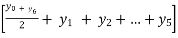
= 1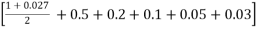
= 1.41
By Simpson’s rule
I = 
= 
= 1.366
Simpson’s  rule
rule 
I = 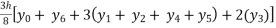
= 
= 1.357
Truncation of error:
The errors that result from using an approximation in place of an exact mathematical procedure
Ex:

 approximation truncation errors
example 1:
maclurian series ln(1+x)
S = 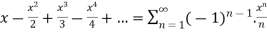 (-1 < x
  1)
1)
Solution:
Consider the given maclurian series is ln(1+x)
And assume n=5
S =  (-1 < x
  1)
1)
 s = 1-
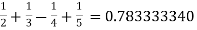
In 2 = 0.693
 =
=
Example 2:
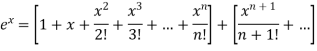
Estimate the truncation error if we calculate e as 
Solution:
Given 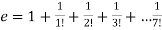
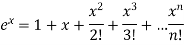
This is the maclurian series of f(x) = ex with x=1 and n=7.
Thus the bound of the truncation error is
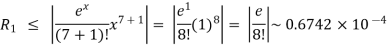
Therefore the actual truncation error is about 0.2786 
Example 3:
How many terms are required in calculation of  using a maclurian series expansion,in which the result is correct to atleast 3 significant figure.
Solution:
Considering the maclurian series
Finding of error for 3 significant values is,

Let equation be 

Then,
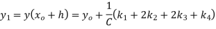

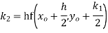
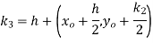
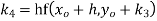
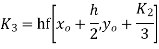
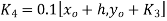
→ Using Runge kutta method of fourth order determine y (0.1) and y(0.2) correct to four decimal place given that  where y(0)=2 and h=0.1.
Ans.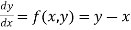
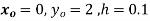
To find y(0.1) we have


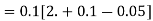

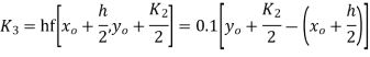
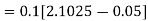


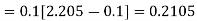
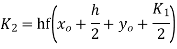
For 


Reference Books:
1. Erwin Kreyszig, “Advanced Engineering Mathematics”, Wiley India,10th Edition.
2. M.D. Greenberg, “Advanced Engineering Mathematics”, Pearson Education, 2 nd Edition.
3. Peter. V and O‟Neil, “Advanced Engineering Mathematics”, Cengage Learning,7th Edition.
4. S.L. Ross, “Differential Equations”, Wiley India, 3rd Edition.
5. S. C. Chapra and R. P. Canale, “Numerical Methods for Engineers”, McGraw-Hill, 7th Edition.
6. J. W. Brown and R. V. Churchill, “Complex Variables and Applications”, McGraw-Hill Inc, 8th Edition.


