Unit - 4
Discrete Fourier Transform
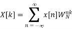
The DTFT of x[n] is defined as follows:
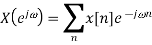
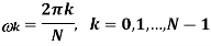
Since ω is a continuous variable, there are an infinite number of possible values of ω from 0 to 2π or from −π to π. Thus, X(ejω) can be computed only at a finite set of frequencies
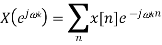
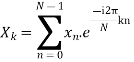
And define the N samples of X(ejω):
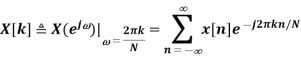
For convenience in notation, we define

However, we still cannot compute X[k] since x[n] can be infinitely long and we are summing for all n. Even if x[n] is finite, we cannot always recover x[n] perfectly from X[k] because X[k]s are essentially the samples of the DTFT. So there are some necessary conditions for which we will be able to recover x[n] from X[k]. In order to find these conditions, first speculate the sampling theorem in the continuous-time domain:
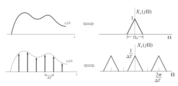
Sampling in time corresponds to replication in the frequency domain. In order to recover Xc(jΩ) perfectly by low-pass filtering Xs(jΩ), frequency aliasing should be avoided. Therefore, x(t) should be bandlimited to Ω0, and sampling interval should be short enough so that

We can apply the time-frequency duality to illustrate the sampling process in the frequency domain. If the sampling interval in frequency is not short enough, we get time aliasing. If the sampling interval in the frequency domain is ΔΩ, it corresponds to replication of signals in time domain at every 2π/ΔΩ. In order to recover x(t) from x˜(t) by time windowing, x(t) should be time-limited to T0, and sampling interval should be small enough so that

We have basically the same result in the discrete-time domain
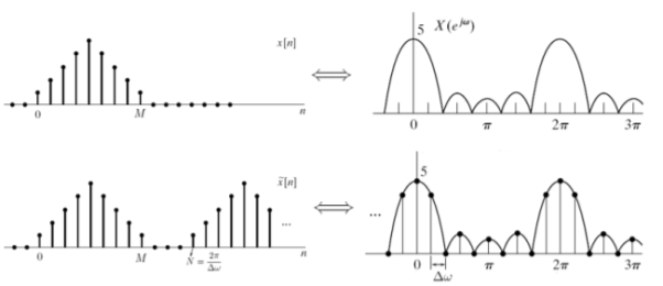
The sampling interval Δω should satisfy the following condition:

If we denote the number of frequency samples from 0 to 2π as N, it is required that

Under this condition, x[n] can be perfectly recovered from the samples of the DTFT:
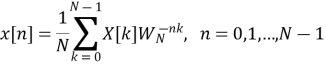
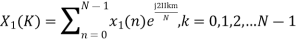
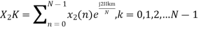
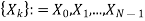
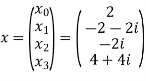
The discrete Fourier transform transforms a sequence of N complex numbers 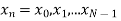 into another sequence of complex numbers
 which is defined by

Example:
Let N =4 and
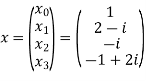
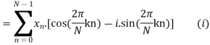
Here we demonstrate how to calculate the DFT of x using equation (1)


The Z transform for discrete time system x(n ) is defined as
X(z) = 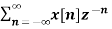 ------- (1) where z is a complex variable.
In polar form z can be expressed as
z = r e jw ---------------(2) where r is the radius of a circle.
For n≥ 0
X(z ) =  --------- (3)which is called one-sided z-transform.
By substituting z = r e jw
X(r e jw) =  (r e jw) –n ------- (4)
 e- jwn ----- (5)
Equation(5) represents the Fourier transform of the signal x(n) r-n
Hence the inverse DTFT X(r ejw) must be x(n) r-n.
x(n) r-n = 1/2π  r e jw ) e jwn dw
On multiplying both sides by rn we get
x(n) = 1/ 2 π  r ejw) (r ejw ) n dw [ z = r ejw
Let z= r e jw and dw= dz/jz
Dz = r ejw dw
Dw = dz/jre jw
Linear Property
If x(t) -> X(w)
Y(t) -> Y(w) then
a x(t) + b y(t) -> a X(w) +b Y(w)
Time Shifting Property
If x(t)⟷F.TX(ω)
Then Time shifting property states that
x(t−t0)⟷F.T e−jω0t X(ω)
Frequency Shifting Property
If x(t)⟷X(ω)
Then frequency shifting property states that
Ejω0t.x(t)⟷X(ω−ω0)
Time Reversal Property
If x(t)⟷X(ω)
Then Time reversal property states that
x(−t)⟷X(−ω)
Differentiation Property
If x(t)⟷X(ω)
Then Differentiation property states that
Dx(t)dt⟷jω.X(ω)
dnx(t)dtn⟷(jω)n.X(ω)
Integration Property
Integration property states that
∫x(t)dt⟷1jω X(ω)
Then
∭...∫x(t)dt⟷(jω)n X(ω)
Multiplication and Convolution Properties
If x(t)⟷X(ω)
y(t)⟷Y(ω)
Then multiplication property states that
x(t).y(t)⟷X(ω)∗Y(ω)
And convolution property states that
x(t)∗y(t)⟷1/2πX(ω).Y(ω)
Key takeaway
S.No | Property | Time Domain | Frequency Domain |
1. | Linearity |  |  |
2. | Time-shifting |  |  |
3. | Frequency-shifting (modulation) |  |  |
4. | Time reversal |  |  |
5. | Conjugation |  |  |
6. | Time-convolution |  |  |
7. | Frequency-convolution |  |  |
 | Parseval’s relation |  |  |
Examples
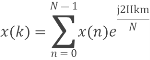
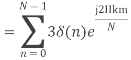
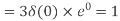
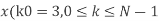
1. Compute the N-point DFT of x(n)=3δ(n).
2. Compute the N-point DFT of x(n)=7(n−n0)
Solution − We know that,
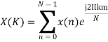
Substituting the value of x(n),
This property is analogous to the time shifting property of the DTFT, but with a subtle difference. Consider length N sequences defined for 0 ≤ n ≤ N – 1. Sample values of such sequences are equal to zero for values of n < 0 and n ≥ N. If x [ n] is such a sequence, then for any arbitrary integer, the shifted sequence
x1[n]= x[n-n0]
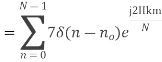
Is no longer defined for the range 0 ≤ n ≤ N – 1. We thus need to define another type of a shift that will always keep the shifted sequence in the range 0 ≤ n ≤ N – 1. The desired shift, called the circular shift, is defined using a modulo operation:
xc[n] =x[(n-no) N]
For (right circular shift), the above equation implies
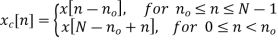
Example of Circular Shift
As can be seen from the previous figure, a right circular shift by no is equivalent to a left circular shift by N-no sample periods. A circular shift by an integer number no greater than N is equivalent to a circular shift by 〈no〉N
The DFT of a sequence can be used to find its finite duration sequence.
We will be proving the property
x(n)  Nx[((-k))N]
Assume that xp(n) is the periodic extension of a discrete-time sequence x(n). If the DFT of x(n) is X(k), we can say that the periodic extension of X(k) is Xp(k)
Thus we can write
xpn  Xp(k)
Xp(k)
Let’s define periodic sequence x1p(n) = Xp(n). Any random single period of this sequence (say x1(n)) will be a finite duration sequence that will be equal to x(n).
The DFT of x1(n), X1(k) is
N xp(-k) for 0<= k <= N-1; and 0 elsewhere
Here N xp(-k) is the discrete Fourier series coefficients of x1p(n). Basically, Nxp(-k) = X1p(k).
X1(k) from the equation above can also be written as
X1(k) = Nx[((-k))]N for 0<= k <= N-1; and 0 elsewhere
Since X1(k) is a DFT of x1(n) and since x1(n) is a finite duration sequence denoted by X(n), we can say that:
x(n)  N x[((-k))N]
Hence, proved
The DFT of an even sequence is purely real and even. DFT of an odd sequence is purely imaginary and odd.
For even sequences:
X(k) =  x(n)Cos(2πnk/N)
For odd sequences:
X(k) =  x(n)Sin(2πnk/N)
X(k) or X(ω) (depending on the expansion notation) is a complex quantity and can be written as:
X(ω) = XR(ω) + jXI(ω)
Where XR(ω) and XI(ω) are the real and imaginary parts of X(ω) respectively.
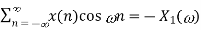
X(ω) = 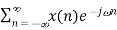
 – j
– j
Comparing the above two equations we have:
XR(ω) = 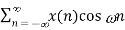
And
XI(ω) = –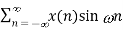
We know that cos(-ω)n = cosωn and sin(-ω)n=-sinωn
Putting -ω to check for even and odd signals
XR(-ω) =
= XR(ω)
Thus
XR(-ω) = XR(ω) (Even and real)
Similarly for the imaginary part we get:
XI(-ω) = 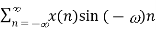 = –
= –
Thus
XI(-ω) = XI(ω) (Odd and imaginary)
Thus we can say
For even sequences:
X(k) =  x(n)Cos(2πnk/N)
For odd sequences:
X(k) =  x(n)Sin(2πnk/N)
Hence, proved.
Let us take two finite duration sequences  ,having integer length as N. Their DI are
  reapectively which is shown below
Now we will try to find the DFT of another sequence  , which is given by
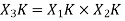
By taking the IDFT of the above we get
After solving the above equation finally we get

Methods of Circular Convolution
Generally, there are two methods, which are adopted to perform circular convolution and they are −
- Concentric circle method,
- Matrix multiplication method.
Concentric Circle Method
Let x1(n) and x2(n) be two given sequences. The steps followed for circular convolution of x1(n) and x2(n) are
- Take two concentric circles. Plot N samples of x1(n) on the circumference of the outer circle maintaining equal distance successive points maintaining equal distance successive points in anti-clockwise direction.
- For plotting x2(n), plot N samples of x2(n) in clockwise direction on the inner circle, starting sample placed at the same point as 0th sample of x1(n)
- Multiply corresponding samples on the two circles and add them to get output.
- Rotate the inner circle anti-clockwise with one sample at a time.
Matrix Multiplication Method
Matrix method represents the two given sequence x1(n) and x2(n) in matrix form.
- One of the given sequences is repeated via circular shift of one sample at a time to form a N X N matrix.
- The other sequence is represented as column matrix.
- The multiplication of two matrices give the result of circular convolution.
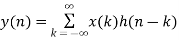
Key takeaway
y(n) = x(n) * h(n)


Examples
Perform circular convolution of the two sequences, x1(n)= {2,1,2,-1} and x2(n)= {1,2,3,4}
Sol:
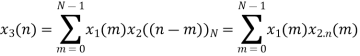
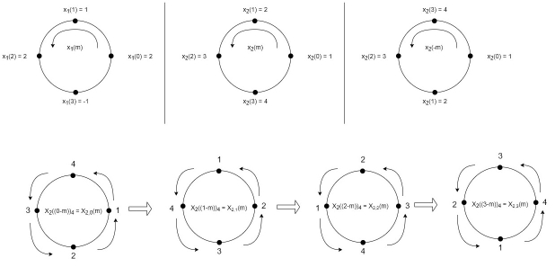
Fig 1 Circular Convolution of x1(n)= {2,1,2,-1} and x2(n)= {1,2,3,4}
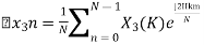
(2)
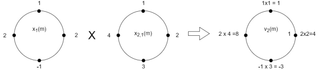
When n=0;
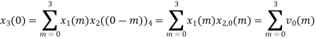
The sum of samples of v0(m) gives x3(0)
⸫ x3(0)=2+4+6-2=10
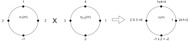
When n=1;
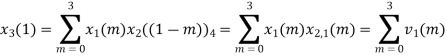
The sum of samples of v1(m) gives x2(1)
⸫ x3(1)=4 + 1 +8-3=10
(3)When n=2; 

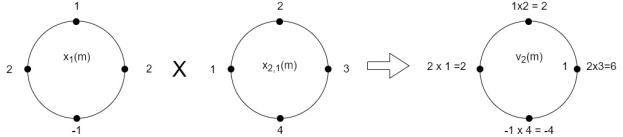
The sum of samples of v2(m) gives x3(2)
⸫ x3(2)=6+2+2-4=6
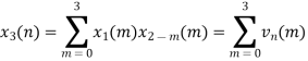
(4) When n=3;


The sum of samples of v3(m) gives x3(3)
⸫ x3(3)=8+ 3+ 4-1= 14
x3(n)={10,10,6,14}

= x1(0) x x2,0(0) + x1(1) x2,0(1) + x1(2) x2,0(2) + x1(3) x2,0(3)
= 2 x 1 + 1 x 4 + 2 x 3 + (-1) x 2 = 2 +4 +6 -2 =10
Linear Convolution states that
y(n) = x(n) * h(n)

Example 1: h(n) = { 1 , 2 , 1, -1 } & x(n) = { 1, 2, 3, 1 } Find y(n).
METHOD 1: GRAPHICAL REPRESENTATION
Step 1) Find the value of n = nx+ nh = -1 (Starting Index of x(n)+ starting index of h(n))
Step 2) y(n)= { y(-1) , y(0) , y(1), y(2), ….} It goes up to length(xn)+ length(yn) -1. i.e n=-1


METHOD 2: MATHEMATICAL FORMULA
Use Convolution formula
k= 0 to 3 (start index to end index of x(n))
y(n) = x(0) h(n) + x(1) h(n-1) + x(2) h(n-2) + x(3) h(n-3)
METHOD 3: VECTOR FORM (TABULATION METHOD)
X(n)= {x1,x2,x3} & h(n) ={ h1,h2,h3}
| X1 | X2 | X3 |
h1 |  |  |  |
h2 |  |  |  |
h3 |  |  |  |
y(-1) = h1 x1
y(0) = h2 x1 + h1 x2
y(1) = h1 x3 + h2x2 + h3 x1 …………
METHOD 4: SIMPLE MULTIPLICATION FORM

The discrete Fourier transform transforms a sequence of N complex numbers  into another sequence of complex numbers
 which is defined by

Example:
Let N =4 and

Here we demonstrate how to calculate the DFT of x using equation (1)


FFT
Certain algorithms permit implementations of Discrete Fourier transform with considerable savings in computation time. These algorithms are known as Fast Fourier Transform.
FFT algorithm are based on fundamental principle of decomposing the computation of DFT of sequence length into successively smaller discrete Fourier transforms.
They are basically two classes of FFT algorithms
- Decimation in time
- Decimation in frequency
Key takeaway
DFT | FFT |
The DFT stands for Discrete Fourier Transform | The FFT stands for Fast Fourier Transform |
The DFT is only applicable for discrete and finite-length signals. Discrete time-domain signals are transformed into discrete frequency domain signals using DFT. | It is an implementation of DFT. |
 | FFT mainly works with computational algorithms for the fast execution of DFT.
|
The time complexity required for a DFT to perform is equal to the order of   | The time complexity reduces in the case of FFT and becomes equal  |
The DFT has less speed than the FFT. | It is the faster version of DFT. |
Some applications of the DFT are spectral analysis, solution of partial differential equations, correlation analysis, etc. | Filtering algorithms, multiplication of integer and polynomials, etc are some applications of the FFT. |
Certain algorithms permit implementations of Discrete Fourier transform with considerable savings in computation time. These algorithms are known as Fast Fourier Transform.
FFT algorithm are based on fundamental principle of decomposing the computation of DFT of sequence length into successively smaller discrete Fourier transforms.
They are basically two classes of FFT algorithms
- Decimation in time
- Decimation in frequency
Decimation-in-time algorithm
This algorithm is known as Radix-2 DIT-FFT algorithm which means the number of output points N can be expressed as a power of 2 that is N = 2M where M is an integer.
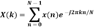
Let x(n) be a sequence where N is assumed to be a power of 2. Decimate or break this sequence into two sequences of length N/2 where one sequence consists of even-indexed values of x(n) and the other of odd-indexed values of x(n).
Xe(n) = x(2n) n= 0,1,……….. N/2-1
Xo(n) = x(2n+1) n= 0,1,……….. N/2 -1
The N-pt DFT of x(n) can be written as
X(k) =  WN nk where k=0,1……….. N-1.
Separating x(n) into even and odd indexed values of x(n) we obtain
X(k) =  WN nk +
  WN nk
WN nk
( n even) (n odd)
=  WN 2nk +
 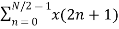 WN (2n+1)k
=  WN 2nk + Wnk
  W N 2nk
X(k) =  WN 2nk + Wnk
  W N 2nk
WN2 =( e-j2π/N) 2 = e-j2π/N/2 = W N/2 .
WN2 = W N/2
X(k) =  W N/2n k + WNk
  WN/2kn
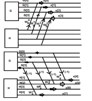
Fig 2 Decimation in time algorithm
W84 = -1
W8 5 = - W 81
W86 = - W82
W87 = - W83
G(0) – H(0) = x(4)
G(1) - W 81 H(1) = x(5)
G(2) - W82 H(2) = x(6)
G(3) - W83 H(3) = x(7)
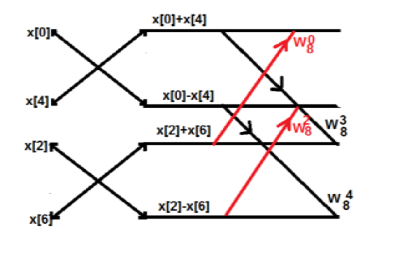
Fig 3 Butterfly Diagram to find W08-W38
Consider the sequence x[n]={ 2,1,-1,-3,0,1,2,1}. Calculate the FFT.
Arrange the sequence as x(0) x(4) x(2) x(6) x(1) x(5) x(3) x(7)
Since N=8 find the values W8 0 to W 87
Apply the butterfly diagram to obtain the values.
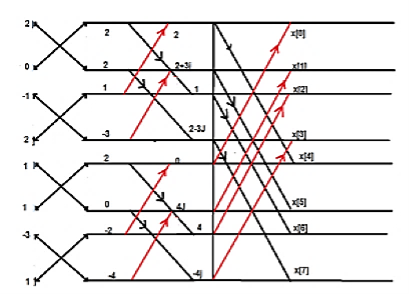
Fig 4 Butterfly Diagram
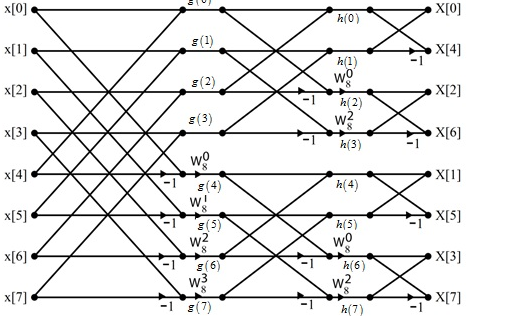
Decimation in Frequency FFT
Apart from time sequence, an N-point sequence can also be represented in frequency. Let us take a four-point sequence to understand it better.
Let the sequence be x[0],x[1],x[2],x[3]………..x[7]
Mathematically, this sequence can be written as;
X(k) =  WN n-k where k=0,1……….. N-1.
Now let us make one group of sequence number 0 to 3 and another group of sequence 4 to 7. Now, mathematically this can be shown as
=  WN nk +
  WN nk
WN nk
Let us replace n by r, where r = 0, 1 , 2….N/2−1.
=  W N/2 nr
We take the first four points x[0],x[1],x[2],x[3] initially, and try to represent them mathematically as follows –
 W 8 nk +
  W8 (n+4) k
=  +
+  W8 (n+4) k
=  + {
+ {  W8 (4) k } W8 nk
X[0] =  + X[n+4]
X[1] =  + X[n+4]) W8 nk
= X(0) – X(4) + (x[1] – X[5]) W8 1 + ( X[2] – X[6] )W82 + X(3) – X(7) W8 3
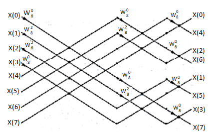
Fig 5 DIF –FFT Algorithm
Find the DIF –FFT of the sequence x(n)= { 1,-1,-1,1,1,1,-1} using Dif-FFT algorithm.
X(0)= 20 X(4) =0
X(1) = -5.828- j2.414 X(5) = -0.1716 + j 0.4141
X(2) = 0 X(6) = 0
X(3) = -0.171 – j 0.4142 X(7) = -5.8284 + j2.4142
Key takeaway
The N-pt DFT of x(n) can be written as
X(k) =  WN nk where k=0,1……….. N-1.
References:
1. Mitra S., “Digital Signal Processing: A Computer Based Approach”, Tata McGraw-Hill,1998, ISBN 0-07-044705-5
2. A.V. Oppenheim, R. W. Schafer, J. R. Buck, “Discrete Time Signal Processing”, 2nd Edition Prentice Hall, ISBN 978-81-317-0492-9
3. Steven W. Smith, “Digital Signal Processing: A Practical Guide for Engineers and Scientists”,1st Edition Elsevier, ISBN: 9780750674447


