Unit - 3
Discrete Time Fourier Transform
Fourier Integral
The formula for the decomposition of a non periodic function into harmonic components whose frequencies range over a continuous set of values.
If a function f(x) satisfies the Dirichlet condition on every finite interval and if the integral
 converges then
F(x) = 1/π 
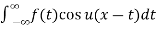 --------- (1)
The formula was first introduced by J. Fourier in connection with the solution of certain heat conduction problems but was proved later by other mathematicians.
Formula(1) can also be given in the form
f(x) = 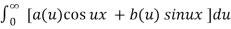 ------- (2)
Where
a(u) = 1/π 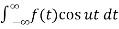
b(u) = 1/π 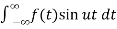
In particular for even functions
f(x) = 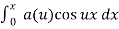 where
where
a(u) = 2/π 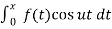
By taking the limits of Fourier series for functions with period 2T as T -> ∞
Then a(u) and b(u) are analogues of the Fourier coefficients of f(x)
Using complex numbers we can replace formula (1) with
f(x) = 1/2π 
 e ju(x-t) f(t)
f(x)= lim 1/π  sin
sin  dt
dt
This is called Fourier Integral.
Problem:
1.Find the Fourier integral of
f(x) = |sin x| |x| ≤ π
= 0 |x| ≥ π
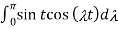
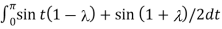
Deduce that  π +1/ 1 -
  2 cos (
 π/2) d
 = π/2
= π/2
Solution:
f(x) = 2/π 

= t
t =
= 
=
= 1/ 1- 2 [cos π + 1]
= π +1/ 1 - 2 cos (π/2) d = π/2
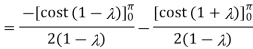
Q. Find the Fourier Integral of
f(x) = 1 |x| ≤ 1
0 |x| ≥ 1
f(x) = 1/π  (t-x) dt d
= 1/π 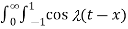 dt d
dt d
= 1/π / ] -1 1 d
= 1/π 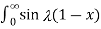 -
-  / d
/ d
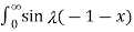
= 1/π  – sin
– sin  ]/ d
]/ d
= 2/π  / d = π/2 when |x| < 1 and 0 when |x| >1
By setting x=0
=  / d = π/2.
Fourier Transform
Consider a periodic signal f(t) with period T. The complex Fourier series representation of f(t) is given as
f(t) =  k ejkw0t
=  k ej2π/T0kt -------- (1)
Let 1/T0 =  f then equation (1) becomes
f(t) =  k ej2π
 kft --------------- (2)
But you know that
Ak = 1/ T0  e-jkw0t dt
Substitute in eq(2)
f(t) = 
 e-jkw0t dt ej2πk
  ft
ft
Let to = T/2 then

 e-j2πkt
  dt ej2πkt
  ft
ft  f
f
As lim T-> ∞  f approaches differential df, k
  f becomes continuous variable hence summation becomes integration
f(t) = lim T-> ∞ { 
 e-j2πk
  ft dt] ej2πk
  ft
ft  f
f
= 
 e-j2π ft dt] ej2π ft df
f(t)= 
 ejwt dw
Where F(w) =  e-j2π ft dt
Fourier transform of a signal is given by
f(t) = F(w) =  e-jwt dt
And Inverse Fourier transform is given by
f(t) =  ejwt dw
Fourier transform are classified into
- Continuous Fourier transform and
- Discrete Fourier transform.
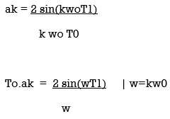
Continuous Fourier Transform
Fourier series was defined for periodic signals. A periodic signals can be considered as a periodic signal with fundamental period
Consider a periodic square wave:
x(t) = 1 for |t| < T1
= 0 T1 < |t| < T0/2
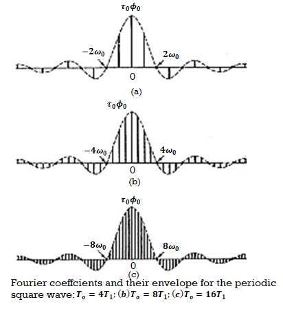
The fourier series co-efficient is
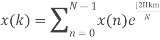
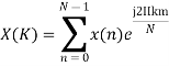
Discrete Fourier Transform
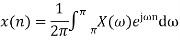
The discrete-time Fourier transform (DTFT) or the Fourier transform of a discrete–time sequence x[n] is a representation of the sequence in terms of the complex exponential sequence ejωn.
The DTFT sequence x[n] is given by
X(w) =  e-jwn ---------------(1)
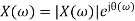
Here X(w) is a complex function of real frequency variable w and can be written as
X(w) = Xre (w) + j X img(w)
Where Xre (w) , j X img(w) are real and Imaginary parts of X(w)
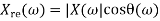
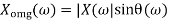
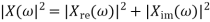
And | X(w)| can be represented as
 .
.
Inverse Discrete Fourier Transform is given by
Problems:
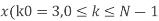
Find the four point DFT of the sequence
x(n) = {0,1,2,3}
Here N=4. W40 = e-j2πn/4 = e-j π/ 2 = cos 0 – j sin = 1 for n=0
W41 = e-j2 π/4 = cos π/2 – j sin π /2 = -j
W42 = e-j π = cos π – j sin π = -1
W43 = e-j2.3 π/4 = cos 3 π/2 – j sin 3 π/2 = j
For k=0
X(k) =  e-j2 π nk/N
X(0) =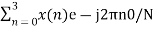
X(0) = x(0)+ x(1)+x(2) + x(3) = 0 +1+2+3 = 6
X(1) =  e-j2 π nk/N
X(1) =  e-j2 π n/4
= x(0) e0 + x(1) e –j2 π /4+ + x(2) e-j4 π/4+ x(3) e- j 6 π/4
= 0 + 1 –j + 2( -1) + 3(j)
= -2+ 2j
X(2) =  e-j2 π n2/4
X(2) =  e-j π n
X(2) = x(0) 1+ x(1) e-j π + x(2) e-j2 π + x(3) e-j3 π
X(2) = -2
X(3) =  e-j2 π n3/4
X(3) = x(0) e0 + x(1) e-j3 π/2 + x(2) e-j3 π + x(3) e-j9 π/2
X(3) = -2-2j.
DFT = { 6, -2+2j,-2,_2-2j}
Properties of Fourier Transform
Linear Property
If x(t) -> X(w)
Y(t) -> Y(w) then
a x(t) + b y(t) -> a X(w) +b Y(w)
Time Shifting Property
If x(t)⟷F.TX(ω)
Then Time shifting property states that
x(t−t0)⟷F.T e−jω0t X(ω)
Frequency Shifting Property
If x(t)⟷X(ω)
Then frequency shifting property states that
Ejω0t.x(t)⟷X(ω−ω0)
Time Reversal Property
If x(t)⟷X(ω)
Then Time reversal property states that
x(−t)⟷X(−ω)
Differentiation Property
If x(t)⟷X(ω)
Then Differentiation property states that
Dx(t)dt⟷jω.X(ω)
dnx(t)dtn⟷(jω)n.X(ω)
Integration Property
Integration property states that
∫x(t)dt⟷1jω X(ω)
Then
∭...∫x(t)dt⟷(jω)n X(ω)
Multiplication and Convolution Properties
If x(t)⟷X(ω)
y(t)⟷Y(ω)
Then multiplication property states that
x(t).y(t)⟷X(ω)∗Y(ω)
And convolution property states that
x(t)∗y(t)⟷1/2πX(ω).Y(ω)
Analysis by Fourier Methods
There are multiple Fourier methods that are used in signal processing.
The most common are
- Fourier transform
- Discrete-time Fourier transform
- Discrete Fourier transform
- Short-time Fourier transform
Key takeaway
Fourier methods are used for two primary purposes:
- Mathematical analysis of problems
- Numerical analysis of data.
- The Fourier transform and discrete-time Fourier transform are mathematical analysis tools and cannot be evaluated exactly in a computer.
- The Fourier transform is used to analyze problems involving continuous-time signals or mixtures of continuous- and discrete-time signals.
- The discrete-time Fourier transform is used to analyze problems involving discrete-time signals or systems.
- In contrast, the discrete Fourier transform is the computational workhorse of signal processing. It is used solely for numerical analysis of data.
- Lastly, the short-time Fourier transform is a variation of the discrete Fourier transform that is used for numerical analysis of data whose frequency content changes with time.
Linear Property
If x(t) -> X(w)
Y(t) -> Y(w) then
a x(t) + b y(t) -> a X(w) +b Y(w)
Time Shifting Property
If x(t)⟷F.TX(ω)
Then Time shifting property states that
x(t−t0)⟷F.T e−jω0t X(ω)
Frequency Shifting Property
If x(t)⟷X(ω)
Then frequency shifting property states that
Ejω0t.x(t)⟷X(ω−ω0)
If x(t)⟷X(ω)
Then Time reversal property states that
x(−t)⟷X(−ω)
If x(t)⟷X(ω)
Then Differentiation property states that
Dx(t)dt ⟷jω.X(ω)
dnx(t)dtn⟷(jω)n.X(ω)
Numerical:
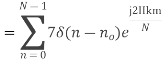
- Compute the N-point DFT of x(n)=3δ(n).
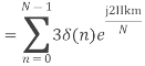
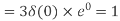
2. Compute the N-point DFT of x(n)=7(n−n0)
Solution − We know that,
Substituting the value of x(n),
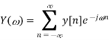
The convolution theorem states that convolution in the time domain is equivalent to multiplication in the frequency domain. Conceptually, we can regard one signal as the input to an LTI system and the other signal as the impulse response of the LTI system. Then, the output spectrum can be calculated by multiplying the input spectrum with the transfer function of the LTI system.
Let x1[n] and x2[n] be two discrete-time signals. If
y[n]= x1[n] * x2[n]
Y(ω) = X1(ω). X2(ω)
Proof
Key takeaway
By duality, multiplication of two signals in the time domain is also equivalent to convolution in the frequency domain. This will be important when we discuss finite-impulse-response (FIR) filter design using the window method
The order of the system is defined as the maximum power of S in the denominator. The type of system is defined as the number of poles at the origin.
For example G(s)= K/S(S+1)
It is order 2 and type 1 system
G(S)= K(S+1)/S2(S+2)
It is order 3 and type 2 system
Standard Test Inputs of Time Domain Analysis
The Impulse signal, Ramp signal, unit step and parabolic signals are used as the standard test signals. All these signals are explained below.
Impulse Signal:
This signal has zero amplitude everywhere except at the origin. Fig below shown the representation of Impulse signal.
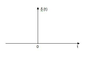
Fig 1 Unit Impulse Signal
The mathematical representations
A (t) = 0 for t ≠0
 dt = A e
Where A represent energy or area of the Laplace Transform of Impulse signal is
L [A (t)] = A
UNIT IMPULSE SIGNAL:
If A = 1
 (t) = 0 for t ≠0
L [ (t)] = 1
The transfer function of a linear time invariant
System is the Laplace transform of the impulse response of the system. If a unit impulse signal is applied to system then Laplace transform of the output c(s) is the transfer function G(s)
As we know G(s) = c(s)/R(S)
r(t) =  (t)
(t)
R(s) = L [ (t)] = 1
:. G(S) = C(s)
(b) Step signal:
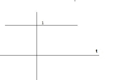
Step signal of size A is a signal that change from zero level to A in zero time and stays there forever.
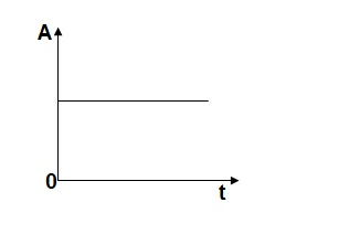
Fig 2 Unit Step Signal
r(t)= A t >=0
=0 t<0
L[r(t)] = R(s) = A/s
UNIT STEP SIGNAL: - If the magnitude of the slip signal is I then it is called unit step signal.
u(t) = 1
t>=0
t<0
L[u(t)] = 1/s
(c) Ramp Signal:
The vamp signal increase linearly with time from initial value of zero at t= 0 as shown in fig is below
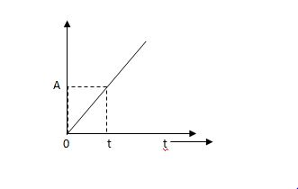
Fig 3 Ramp Signal
r(t) = At t>=0
=0 t<0
A is the slope of the line The Laplace transform of ramp signal is
L[r(t)] = R(s) = A/s2
(d) Parabolic Signal:
The instantaneous value of a parabolic signal varies as square of the time from an initial value of zero t=0. The signal representation in fig 14 below.
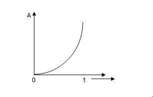
Fig 4 Parabolic Signal
r(t) At2 t>=0
=0 t<0
Then Laplace Transform is given as
R(s) = L[At2] = 2A/s3
If no error then E(t) =0, :. R(t) = c(t), output is tracking the input.
Steady state Errors signal (ess): - (t  )
)
Ess = t  e(t)
e(t)
Using final values, the theorem
 = ess =
  S.E (s)
ess=  S[R(s)/1+G/(s)]
First Order System:
OLTF G(s) = 1/TS
CLTF c(s)/R(s) = 1/1+TS
CE: HTS = 0
S= -1/T
C(s) = R(s) [G(S)/1+G(s)]
C(s) = R(s)/1+TS
So, Calculating value of c(s), c(t) for different input
a) Unit Step:
R(t) = u(t)
R(s) = 1/s
C(s) = 1/s(1+ST)
1/s(1+ST) = A/s + o/1+TS
1/s(1+ST) = A/S + 0/1+TS
1= A(1+ST) + BS
AT +B =0
A = 1
B= -T
C(s) = 1/s + (-T)/1+TS
= 1+ (-T)/1-(-T)s = 1-I/n/1+ass+1/T =e-t/s
C(t) = [ 1-e-t/T]
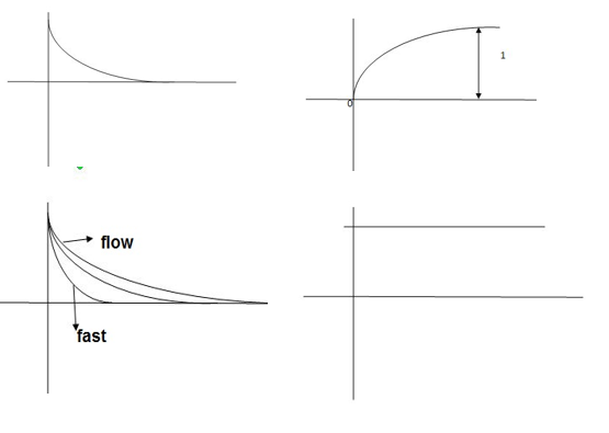
Fig 5 Output response for Unit Step input
Ramp:
R(t) = t
R(s) = 1/s2
C(s) = R(s) [G(s)/1+G(s)]
C(s) = 1/s2 1/(1+TS) + c
1/s2 (1+TS) = A/(s) + B/s2 + c(1+TS)
1= A (s+s2. T) + B(1+TS) +cs2
TA +c = 0
A+TB =0
B =1
A = -T
C = T2
C(s) = -T/s + 1/s2 +T2/1+ST
=(-T) u(t) + t(u) + T e-t/T u(t)
= [ -T + t +Te-t/T u(t)
= [ -T+ t+Te-t/T] u(t)
C(s) = t- T+ Te-t/T
ess =  R(t) – c(t)
=  [ t- t+ 7-Te –t/T]
=  T( 1-e-t/T]
ess = The less the value of T the less in the errors.
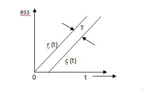
Fig 6 Output response for ramp input
From both the Cases input unit step, ramp Unit step
Unit Step Ramp
c(t) = 1-e-t/T r(t) = t
ess = e-t/T (r/t)-(t) c(t) = t- T+te-t/T
ess= e-t/T (r/t) (t) ess = T- Te-t/T
For :- for
 :-
:-
ess =0 ess = T
1) In both the vases (values of T) must be as small as possible (so, that e-t/T) must be as small as possible which gives us
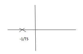
Fig 7 Location of poles
G(s) = 1/Ts
ATf = 1/1+TS
1st order system
Poles must be situated as far as possible from origin i.e. deeper and deeper into the left half of s-place. Thus, we get less errors.
Second Order System:
OLTF G(s) = k/s(1+TS)
CLTFC(s)/R(s) = k/k+s(1+Ts)
= k/s2+ s/T +k/T
Comparing above equation with standard 2nd order eqn
CLTF = wn2/s2+2rs wns+wn2 standard 2nd order equation
CEs2+2 wn s+wn2 = 0
S= -2 wn±
wn± /2
/2
=2 wn±2wn
 /2
/2
S= wn±wn
wn±wn
S= - wn±wn
wn±wn
S= - wn ±wn
S= - wn ±gwn
Standard eqn:
T(s) = wn2/s2+2 wns+wn2
Our eqn T(s) = K/T/s2+1/T s+ K/T
Wn2 = k/T
2 wn = 1/T
2 k/T = 1/T
 k/T = 1/2T
 = 1/2T
  T/K
T/K
 = 1
= 1 2KT
2KT
Graphically showing the position of loops s1,s2 for offered of
As the characteristic Eqn (location of poles) is dependent only on (wn constant for a given system)
S1 = - wn + jwn
  1-
1- 2
2
S2= - wn - jwn
 1-
1- 2
2
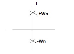
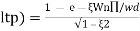
CASE 1: ( =0)
=0)
S1=jwn,S2, = -jwn
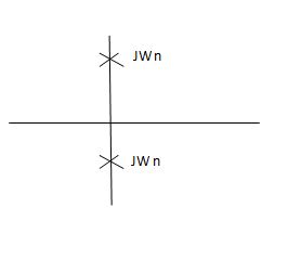
Fig 8 Location of poles for  =0
=0
Undamped
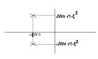
CASE 2:(0< <1)
<1)
S1= -wn + jwn  0.75
0.75
=-wn/2 +jwn(0.26)
S2 = -wn/2 – jwn (0.86)
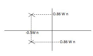
Fig 9 Location of poles for  <1
<1
CASE:3 ( =1)
=1)
S1= S2 = - wn = -wn
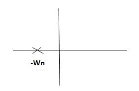
Fig 10 Location of poles for  =1
=1
CASE4: ( =-2)
=-2)
S1 = -2wn +jwn  -3
-3
=-2wn – jwn (1.73)
S1 = -3.73wn
S2 = -2wn –jwn  -3
-3
= -2wn + jwn (1.73)
= -0.27  wn
wn
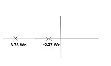
Fig 11 Location of poles for  >1
>1
Overdamped
All practical systems are 2 order to, if R(e) =  (t)
(t)
:. CLTF = 2nd order st equation and hence already the system is possible.
CLTF = e(s)/ R(s) = wn2/s2+2 wns+wn2
Now calculating c(s), c(t) for different values of input
1) Impulse I/p
R(t) =  (t)
(t)
R(s) = 1
C(s) = R(s) wn2/s2+2 wns+wn2
C(s) = wn2/s2 +2 wn+wn2
Under this i/p (R(t) =  (t)) the output varies with different values of
  . So,
. So,
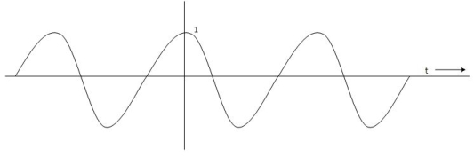
CONDITION 1: ( =0)
=0)
C(s) =wn2/s2 +wn2
Os2 +wn2 =0
S=+-jwn
C(t) = wn sinwnt
Sinwnt
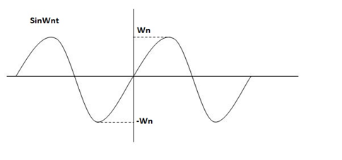
Fig 12 Undamped oscillations
As there in no damping i.e. oscillations at t= 0 are some at t  so, called UNDAMPED
CONDITION 2: 0<<1
c(s) = R(s) wn2/s22 wn+wn2 R(t) =
  (t)
(t)
R(s) =1
C(s) = wn2/s2+2 wns+wn2
CE
S2+2 wns +wn2 =0
S2, S1 = - wn ±jwn
  1-
1- 2
2
C(t) = e- wnt sin( wn
  )t
)t
Wd=wn )
)
C(t)=e- wnt sin (wdt)
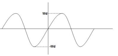
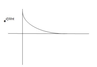
Fig 13 Underdamped oscillations
The oscillations are present but at t- infinity the Oscillations are 0 so, it is UNDERDAMPED
CONDITION 3:  =1
=1
C(s) = R(s) wn2/s2+2 wns+wn2
C(s)=wn2/S2 +2wns+wn2
=wn2/(s +wn)2
CE S= -Wn
Diagram
C(t)= w2n /(
 )2
)2
C(t)=
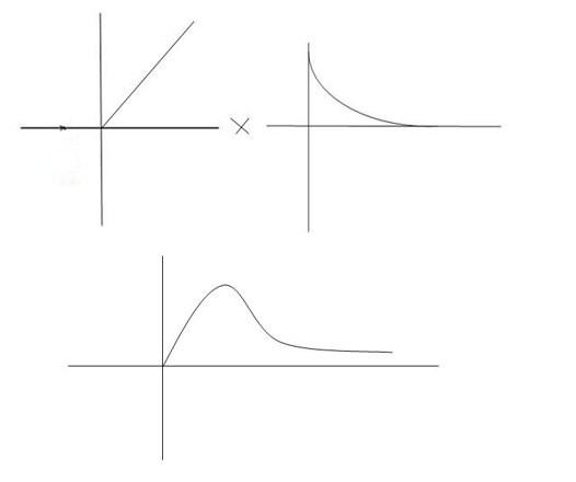
Fig 14 Critically damped oscillations
No damping obtained at  so is called CRITICALLY DAMPED.
CONDITIONS 4: >1
>1
C(s) = wn2/s22 wnS+Wn2
S1, s2 =  WN+-jwn
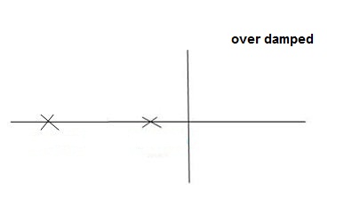
Fig 15 location of poles for over damped oscillations
b) UNIT Step Input:
R(s) = 1/s
C(s)/R(s) = wn2/s2+2 wns+wn2
C(s) = R(s) wn2 /s2 +2 wns+wn2
C(s) = R(s) wn2/s2+2 wns+wn2
C(s) = R(s) wn2/s2+2 wns+wn2
C(s) = wn2s(s2+2 wns+wn2)
C(t) = 1- e wnt/
wnt/ 1-es2 sin (wdt + ø)
Wd = wn 1-
1- 2
2
Ø= 
Where
Wd = Damping frequency of oscillations
Wn = natural frequency of oscillations
 wn = damping coefficient.
T= Time constant
Condition 1 = 0
= 0
C(s) = wn2 /s(s2+wn2)
C(t) = 1- e° sin wdt +ø
C(t)= 1- sin( wn +90)
C(t) = 1+cos wnt
Constant
C(t) = 1+constant
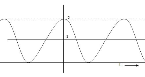
Fig 16 C(t) = 1+cos wnt
Condition 2: 0< <1
<1
C(s) =  /s2+
/s2+ wns +wn2
C(s) =1/s – s+ wn/s2+
 wns +wn2
=1/s – s+ wn/(s+
 wn)2+wd2-
  wn/(s+
 wn2) +wd2
Wd = wn  1-
1- 2
2
Taking Laplace inverse of above equation
L --1 s+ wn/(s+
 wn) +wd2= e-
 wnt cos wdt
L-1 s+ wn/(s+
 wn)2+wd2 = e-
 wnt sinWdt
C(t) = 1-e- wnt [coswdt +
 /
/ 1-
1- 2 sinwdt]
= 1-e wnt /
wnt / 1-
1- 2 sin [wdt +
  1-
1- 2/
2/ ] t>=0
C(t) = 1-e wnt/
wnt/ 1-
1- 2 sin(wdt+ø)
Ø =  1+
1+ 2/
2/
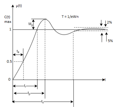
Fig 17. Transient Response of second order system
Specifications:
1) Rise Time (tp): The time taken by the output to reach the already status value for the first time is known as Rise time.
C(t) = 1-e- wnt/
wnt/ 1-
1- 2 sin (wdt+ø)
Sin (wd +ø) = 0
Wdt +ø = n
tr =n -ø/wd
-ø/wd
For first time so n=1.
tr =  -ø/wd
-ø/wd
T=1/
2) Peak Time (tp)
The peak value attained by the output is called peak time. The time required by the output to reach this value is lp.
d(cct) /dt = 0 (maxima)
d(t)/dt = peak value
tp = n /wd for n=1
tp =  wd
wd
3) Peak Overshoot Value:
Maximum deviation of output from steady state value is called peak overshoot value (Mp).
(ltp) = 1 = Mp
( Sin(Wat + φ )
( Sin( Wd∏/Wd + φ)
Mp = e-∏ξ / √1 –ξ2
Condition 3 ξ = 1
C( S ) = R( S ) Wn2 / S2 + 2ξWnS + Wn2
C( S ) = Wn2 / S(S2 + 2WnS + Wn2) [ R(S) = 1/S ]
C( S ) = Wn2 / S( S2 + Wn2 )
C( t ) = 1 – e-Wnt + tWne-Wnt
The response is critically damped.
(4). Settling Time (ts):
ts = 3 / ξWn ( 5% )
ts = 4 / ξWn ( 2% )
Key takeaway
For a second order control system, the total time response is analyzed by its transient as well as ready state response.
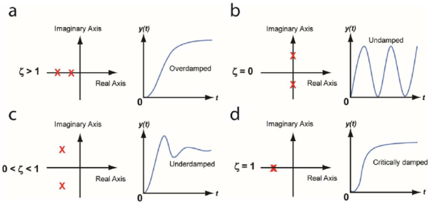
Any system which contains energy along elements (L1 c etc) if suffer any disturbance in the energy state effect at the input end as at this output or at both the ends takes source time to change in thus form one state other . This change its then is called as Transient times and the values of reverent and voltage during this period is Transient Response.
The above fig: a clearly shows steady star response is that part of response when the transient have died. If the steady star response of the output does not match with input then the system has steady state errors.
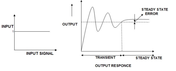
Consider the following open loop system
L-1[c(s)]= L-1[ G(s) R (S)]
C(t) = L-1[ G(S) Q (s)]
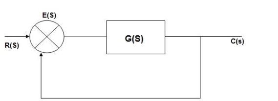
E(s) = R(s) –c(s) [ error signal]
C(S)= [ R(s)- c(Q)] G(s)
C(s) = R(s) G(s)- c(s) G(s)
C(s) [ 1+G(s)] = R(s) G(s)
C(s)/R(s) = G(s)/1+G(s)
C(s)/R(s) = G(s)/1+G(s)
E(s) = R(s)- c(s)
=R(s)-R(s) G(s)/1+G(s0
E(s) = R(s) [1/1+G(s)
If no error then E(s) = 0, f(t) = 0 Hence, r(t) = c(t)
Key takeaway
The error signal is the difference between the unity feedback signal and input signal.
Examples
Q.1. The open loop transfer function of a system with unity feedback gain G( S ) = 20 / S2 + 5S + 4. Determine the ξ, Mp, tr, tp.
Sol: Finding closed loop transfer function,
C( S ) / R( S ) = G( S ) / 1 + G( S ) + H( S )
As it is unity feedback so, H(S) = 1
C(S)/R(S) = G(S)/1 + G(S)
= 20/S2 + 5S + 4/1 + 20/S2 + 5S + 4
C(S)/R(S) = 20/S2 + 5S + 24
Standard equation for second order system,
S2 + 2ξWnS + Wn2 = 0
We have,
S2 + 5S + 24 = 0
Wn2 = 24
Wn = 4.89 rad/sec
2ξWn = 5
(a). ξ = 5/2 x 4.89 = 0.511
(b). Mp% = e-∏ξ / √1 –ξ2 x 100
= e-∏ x 0.511 / √1 – (0.511)2 x 100
Mp% = 15.4%
(c). tr = ∏ - φ / Wd
φ = tan-1√1 – ξ2 / ξ
φ= tan-1√1 – (0.511)2 / (0.511)
φ = 1.03 rad.
tr = ∏ - 1.03/Wd
Wd = Wn√1 – ξ2
= 4.89 √1 – (0.511)2
Wd = 4.20 rad/sec
tr = ∏ - 1.03/4.20
tr = 502.34 msec
(d). tp = ∏/4.20 = 747.9 msec
Q.2. A second order system has Wn = 5 rad/sec and is ξ = 0.7 subjected to unit step input. Find (i) closed loop transfer function. (ii) Peak time (iii) Rise time (iv) Settling time (v) Peak overshoot.
Sol: The closed loop transfer function is
C(S)/R(S) = Wn2 / S2 + 2ξWnS + Wn2
= (5)2 / S2 + 2 x 0.7 x S + (5)2
C(S)/R(S) = 25 / S2 + 7s + 25
(ii). tp = ∏ / Wd
Wd = Wn√1 - ξ2
= 5√1 – (0.7)2
= 3.571 sec
(iii). tr = ∏ - φ/Wd
φ= tan-1√1 – ξ2 / ξ = 0.795 rad
tr = ∏ - 0.795 / 3.571
tr = 0.657 sec
(iv). For 2% settling time
ts = 4 / ξWn = 4 / 0.7 x 5
ts = 1.143 sec
(v). Mp = e-∏ξ / √1 –ξ2 x 100
Mp = 4.59%
Q.3. The open loop transfer function of a unity feedback control system is given by
G(S) = K/S(1 + ST)
Calculate the value by which k should be multiplied so that damping ratio is increased from 0.2 to 0.4?
Sol: C(S)/R(S) = G(S) / 1 + G(S)H(S) H(S) = 1
C(S)/R(S) = K/S(1 + ST) / 1 + K/S(1 + ST)
C(S)/R(S) = K/S(1 + ST) + K
C(S)/R(S) = K/T / S2 + S/T + K/T
For second order system,
S2 + 2ξWnS + Wn2
2ξWn = 1/T
ξ = 1/2WnT
Wn2 = K/T
Wn =√K/T
ξ = 1 / 2√K/T T
ξ = 1 / 2 √KT
Forξ1 = 0.2, for ξ2 = 0.4
ξ1 = 1 / 2 √K1T
ξ2 = 1 / 2 √K2T
ξ1/ ξ2 = √K2/K1
K2/K1 = (0.2/0.4)2
K2/K1 = 1 / 4
K1 = 4K2
Q.4. Consider the transfer function C(S)/R(S) = Wn2 / S2 + 2ξWnS + Wn2
Find ξ, Wn so that the system responds to a step input with 5% overshoot and settling time of 4 sec?
Sol:
Mp = 5% = 0.05
Mp = e-∏ξ / √1 –ξ2
0.05 = e-∏ξ / √1 –ξ2
Cn 0.05 = - ∏ξ / √1 –ξ2
-2.99 = - ∏ξ / √1 –ξ2
8.97(1 – ξ2) = ξ2∏2
0.91 – 0.91 ξ2 = ξ2
0.91 = 1.91 ξ2
ξ2 = 0.69
(ii). ts = 4/ ξWn
4 = 4/ ξWn
Wn = 1/ ξ = 1/ 0.69
Wn = 1.45 rad/sec
Q5) Find the initial value for the function f(t) = 2u(t)+3cost u(t)?
Sol:
f(t) = 2u(t)+3cost u(t)
F(s) = 
SF(s) = 2+ 
By initial value theorem
 = f(0+)
 =
=  2+
2+  = 5 = f(0+)
Hence, initial value of the function is 5
Q6) Find final value of the function F(s) = 
Sol:
F(s) = 
SF(s) = 
By final value theorem
 =
= 
 =
=  = 0.1
= 0.1
So, final value of the function is 0.1
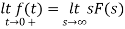
Key takeaway
By initial value theorem
 = f(0+)
By final value theorem
 =
= 
References:
1. Mitra S., “Digital Signal Processing: A Computer Based Approach”, Tata McGraw-Hill,1998, ISBN 0-07-044705-5
2. A.V. Oppenheim, R. W. Schafer, J. R. Buck, “Discrete Time Signal Processing”, 2nd Edition Prentice Hall, ISBN 978-81-317-0492-9
3. Steven W. Smith, “Digital Signal Processing: A Practical Guide for Engineers and Scientists”,1st Edition Elsevier, ISBN: 9780750674447


