Unit - 1
Discrete-time signals and systems
Analog
Analog signals are continuous in time. A continuous-time signal is an infinite and uncountable sequence of numbers, as are the possible values each number can have. – between a start and end time, there are infinite possible values for time t and the waveform’s instantaneous amplitude x(t). A continuous signal cannot be stored, or processed, in a computer since it would require infinite data. Analog signals must be discretized (digitized) to produce a finite set of numbers for computer use.
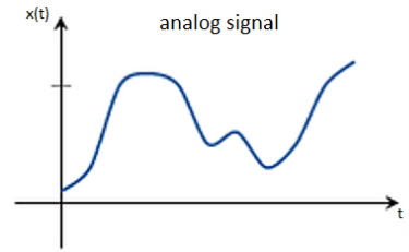
Fig 1 Analog Signal
A signal, of which a sinusoid is only one example, is a set, or sequence of numbers. The term “analog” refers to the fact that it is “analogous” of the signal it represents. A “real-world” signal is captured using a microphone which has a diaphragm that is pushed back and forth according to the compression and rarefaction of the sounding pressure waveform. The microphone transforms this displacement into a time-varying voltage—an analog electrical signal.
Discrete-time signals
If a discrete variable x(t) is defined at discrete time then x(t) is a discrete time signal. A discrete time signal is often identified as a sequence of number denoted by x(n), where ‘n’ is an integer.
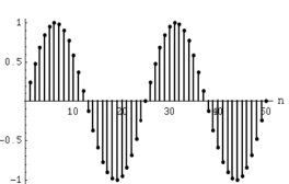
Fig:2 Discrete time signal
Digital signals
A digital signal carries data in discrete form which are represented in binary bits. They can be decomposed into sine waves called as harmonics. These signals have specific frequency, amplitude and phase. They are mostly defined by the bit rate in given bit intervals. The time required to transmit one bit is called as bit rate. They are more efficient when it comes to noise. They are represented in 1 and 0 form.
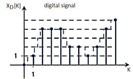
Fig 3 Digital Signal
Key takeaway
S.No | Discrete-time signal | Digital signal |
1. | The discrete-time signal is a digital representation of a continuous time signal. | The digital signal is form of discrete-time signal. |
2. | The discrete-time signal can be obtained from the continuous-time signal by the Euler’s method. | The digital signal can be obtained by the process of sampling, quantizations, and encoding of the discrete-time signal. |
3. | The discrete-time signal sia signal that has discrete in time and discrete in amplitude. | The digital signal is a signal that has discrete in amplitude and continuous in time. |
4 | The value of the signal can be obtained only at sampling instants of time. | The amplitude signal of the digital signal is either 1 or 0. That is either OFF or ON. |
5 | The signals are sampled but not necessary to quantized in the discrete-time signals. | The signals are sampled and quantized in the digital signals. |
6. | All the discrete-time signals are digital signals. | All the digital signals are not discrete-time signals. |
S.No | Analog signal | Digital signal |
1 | Analog signals are continuous signals. | Digital signals are discrete signals. |
2 | Analog signal uses continuous values for representing the information. | A digital signal uses discrete values for representing the formation. |
3. | Analog signal uses continuous vlaues for representing the information. | A digital signal cannot be affected by the noise during transmission. |
4 | Accuracy of Analog signal is affected by the noise. | Digital signals are noise-immune hence there accuracy is less affected. |
5 | Devices which are using analog signals are less flexible | Device using digital signals are very flexible. |
6 | Analog signals consumes less bndwidth | Digital signals consume more bandwidth |
7 | Analog signal are stored in the form of continuous wave form. | Digital signals are stored in the form of binary bits “0”, “1”. |
9 | Analog signals have low cost. | Digital signals have high cost. |
10 | Analog signals give observation error. | Digital signals doen’t give observaiton error. |
Basic sequences
Unit sample sequence
δ(n) = 1, n = 0
=0, n 0
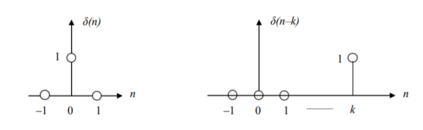
Fig 4 Unit Sample Sequence
Whereas δ(n) is somewhat similar to the continuous-time impulse function δ(t) – the Dirac delta – we note that the magnitude of the discrete impulse is finite. Thus there are no analytical difficulties in defining δ(n). It is convenient to interpret the delta function as follows:
δ(argument) = 1 when argument 0
= 0 when argument ≠ 0
The unit step sequence
u(n) = 1, n 0
=0, n < 0
u(argument) = 1, if argument 0
=0, if argument < 0
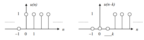
Fig 5 Unit Step Sequence
a) The discrete delta function can be expressed as the first difference of the unit step function:
δ(n) = u(n) – u(n–1)
b) The sum from – to ‘n’ of the δ function gives the unit-step:
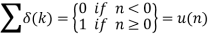
Results (a) and (b) are like the continuous-time derivative and integral respectively.
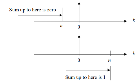
Exponential sequence
Consider the familiar continuous time signal x(t) = e t = e t / , t 0
The sampled version is given by setting t = nT
x(nT) = e n T = e Tn, nT 0
Dropping the T from x(nT) and setting e T = a
We can write x(n) = an, n 0
The sequence can also be defined for both positive and negative n, by simply writing x(n) = an for all n.
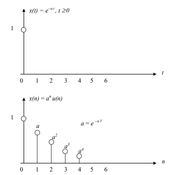
Fig 6 Exponential Sequence
Sinusoidal sequence
Consider the continuous-time sinusoid x(t)
x(t) = A sin 2πF0t = A sin Ω0t
F0 and Ω0 are the analog frequency in Hertz (or cycles per second) and radians per second, respectively. The sampled version is given by
x(nT) = A sin 2πF0nT = A sin Ω0nT
We may drop the T from x(nT) and write
x(n) = A sin 2πF0nT = A sin Ω0nT, for all n
We may write Ω0T = ω0 which is the digital frequency in radians (per sample), so that
x(n) = A sin ω0n = A sin 2πf0n, for all n
Setting ω0 = 2πf0 gives f0 = ω0/2π which is the digital frequency in cycles per sample. In the analog domain the horizontal axis is calibrated in seconds; ―second, is one unit of the independent variable, so Ω0 and F0 are in ―per second. In the digital domain the horizontal axis is calibrated in samples; ―sample is one unit of the independent variable, so ω0 and f0 are in ―per sample.
Sequence operations
Shifting and folding (reflecting about the vertical axis) Given the sequence x(n), where n is the independent variable, we have the following two transformation operations:
Shifting in time by k units, where k is an integer, is denoted by x(n–k). The sequence x(n–k) represents the sequence x(n) shifted by k samples, to the right if k is positive, or to the left if k is negative. Parenthesize n and replace it by (n–k) for k units of delay, or by (n+k) for k units of time advancement.
Folding (a.k.a. Time reversal or reflecting about the vertical axis) is denoted by x(–n). The signal x(–n) corresponds to reflecting x(n) about the time origin n = 0. Reverse the sign of n (replace n with –n).
Given the delta function δ(n), first reflect then shift (delay) by 2 units. The other possibility is first to shift (delay) by 2 units and then reflect. The result of ―reflect then shift is shown below left. Reflect means to change the sign of n; then shifting is done by replacing (n) by (n–2).
The result is: (1) δ(n)‹δ(–n) and (2) δ(–n) = δ(–(n)) < δ(–(n–2)) = δ(–n+2).
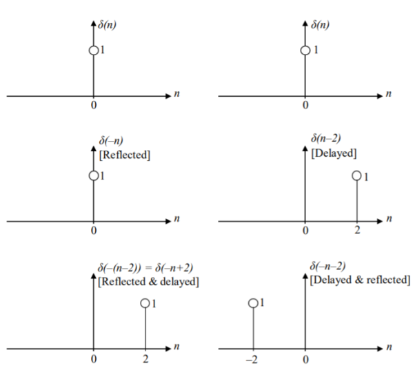
To continue the example, the second possibility, the result of ―shift then reflect is shown above right. Shift means replacing (n) by (n–2); then reflect by changing the sign of n. The result is δ(– n–2). The result is: (1) δ(n) = δ((n)) < δ((n–2)) and (2) δ((n–2)) = δ(n–2) ‹ δ(–n–2). Note that the two end results are not the same.
Time Delayed Signal
When the signal is moved towards right with keeping its amplitude same but we just move the signal three units towards right. If y[n] =x[n] then if we move the signal three units towards right, we can write y[n] = x[n-3]
Time Advanced Signal
It is reverse of the above case. Here we move signal towards the left keeping it’s amplitude same. If we move the signal four units towards the left then
Y[n] =x[n+4]
Time Scaling
Time scaling refers to the multiplication of the variable by a real positive constant.
If a > 1 the signal y(t) is a compressed version of x(t).
If 0 < a < 1 the signal y(t) is an expanded version of x(t).
y(t) = x(at)
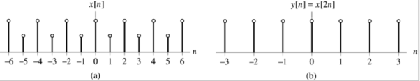
In the discrete time
y[n] = x[kn],
It is defined for integer value of k, k > 1. Figure below for k = 2, sample for n = +-1,
Key takeaway
This serves to illustrate that the two operations of shifting and reflecting are not commutative: Fold (Shift(δ(n))) ≠ Shift (Fold(δ(n)))
If you have Time shifting and Reversal together. First Shift then Reverse.
Examples
Q) Determine if the system y(n) = T[x(n)] = x(–n) is linear or nonlinear.
A) Determine the outputs y1(.) and y2(.) corresponding to the two input sequences x1(n) and x2(n) and form the weighted sum of outputs:
y1(n) = T[x1(n)] = x1(–n) y2(n) = T[x2(n)] = x2(–n)
The weighted sum of outputs = a1 x1(–n) + a2 x2(–n) ‹(A).
Next determine the output y3 due to a weighted sum of inputs:
y3(n) = T[a1 x1(n) + a2 x2(n)] = a1 x1(–n) + a2 x2(–n) <(B)
Check if (A) and (B) are equal. In this case (A) and (B) are equal; hence the system is linear.
Q) Examine y(n) = T[x(n)] = x(n) + n x(n+1) for linearity.
A) The outputs due to x1(n) and x2(n) are:
y1(n) = T[x1(n)] = x1(n) + n x1(n+1)
y2(n) = T[x2(n)] = x2(n) + n x2(n+1)
The weighted sum of outputs = a1 x1(n) + a1 n x1(n+1) + a2 x2(n) + a2 n x2(n+1) <(A)
The output due to a weighted sum of inputs is
y3(n) = T[a1 x1(n) + a2 x2(n)]
= a1 x1(n) + a2 x2(n) + n (a1 x1(n+1) + a2 x2(n+1))
= a1 x1(n) + a2 x2(n) + n a1 x1(n+1) + n a2 x2(n+1) <(B)
Since (A) and (B) are equal the system is linear.
Q) Check the system y(n) = T[x(n)] = ne |x(n)| for linearity.
A) The outputs due x1(n) and x2(n) are:
y1(n) = T[x1(n)]= n e |x1 (n)|
y2(n) = T[x2(n)] = n e|x2 (n)|
The weighted sum of the outputs = a1 ne|x1 (n)|+ a n e|x2 (n)| <(A)
The output due to a weighted sum of inputs is y3(n) =T[a1 x1(n) + a2 x2(n)] = n e|a1 x1 (n)|+|a2x1 (n)| <(B) We can specify a1, a2, x1(n), x2(n) such that (A) and (B) are not equal. Hence nonlinear.
Q) Check the system y(n) = T[x(n)] = n x(n) for linearity.
A) For the two arbitrary inputs x1(n) and x2(n) the outputs are
y1(n) = T[x1(n)] = n x1(n)
y2(n) = T[x2(n)] = n x2(n)
For the weighted sum of inputs a1 x1(n) + a2 x2(n) the output is
y3(n) = T [a1 x1(n) + a2 x2(n)] = n (a1 x1(n) + a2 x2(n)) = a1 n x1(n) + a2 n x2(n) = a1 y1(n) + a2 y2(n). Hence the system is linear.
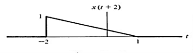
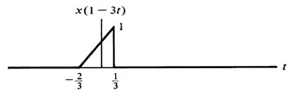
Q) For x(t) indicated in figure 1 sketch the following
(a) x(-t)
(b) x(t+2)
(c) x(2t+2)
(d) x(1-3t)
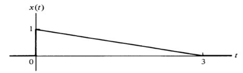
A)
(a) This is just a time reversal
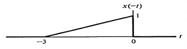
Note: Amplitude remains the same. Also reversal occurs about t=0
(b) This is a shift in time. At t=-2, the vertical portion occurs.
(c)A scaling by a factor of 2 occurs as well as time shift

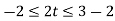


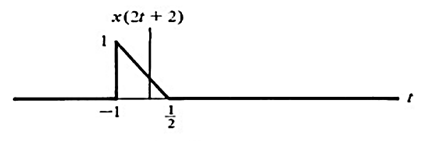
Note: a>1 induces a compression
(d) All three effects are combined in this linear scaling.


A discrete-time system is anything that takes a discrete-time signal as input and generates a discrete-time signal as output. The concept of a system is very general. It may be used to model the response of an audio equalizer or the performance of the US economy. In electrical engineering, continuous-time signals are usually processed by electrical circuits described by differential equations.
For example, any circuit of resistors, capacitors and inductors can be analysed using mesh analysis to yield a system of differential equations. The voltages and currents in the circuit may then be computed by solving the equations. The processing of discrete-time signals is performed by discrete-time systems. Similar to the continuous-time case, we may represent a discrete-time system either by a set of difference equations or by a block diagram of its implementation. For example, consider the following difference equation.
y[n] = y[n − 1] − 2x[n] + 3x[n − 1]
This equation represents a discrete-time system. It operates on the input signal x[n] to produce the output signal y[n]. This system may also be defined by a system diagram as in Figure.
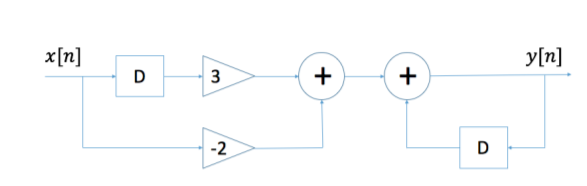
Fig:7 Diagram of a discrete-time system.
Discrete-time digital systems are often used in place of analog processing systems. Common examples are the replacement of photographs with digital images, and conventional NTSC TV with direct broadcast digital TV. These digital systems can provide higher quality and/or lower cost through the use of standardized, high-volume digital processors.
1) Linear and Non-Linear system:
A system is said to be linear when it obeys law of superposition.
If we have two inputs x1(n) and x2(n), and output y(n). The operator ‘H’ is called linear operator if it satisfies the following condition.
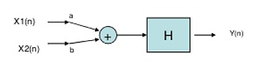
Fig 8 Input first pass through adder
In the above figure first the two inputs pass through an adder than through the operator. So, the equation after adder will be ax1(n)+bx2(n). Now final output equation after passing through operator is
Y(n)=H[ax1(n)+bx2(n)]=Hax1(n)+H bx2(n)
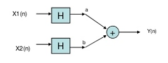
Fig 9 Input first pass through operator
Now, in above figure the two inputs first pass through the operator and then through the summer. The equation at output is
Y(n)= Hax1(n)+H bx2(n)
The two output equations in both the systems are same. Hence, the system operator H is linear.
Non-Linear system: If the system does not obey law of superposition, it is said to be non-linear.
2) Time variant and Time Invariant system: A time delay or advance in the input signal produces the corresponding change in the output. Then the system is said to be time invariant.


If the delay or advance in the system does not produce corresponding change in the output then it’s called as Time variant System.
3) Causal and Anti-Causal system: A system is said to be causal if it’s output at any point of time depends only on the input x(t) for time ‘t’, where t<t0, where t0 is the present time. If not so then it is called as anti-causal system.
Only causal signals are realisable signals.
4) Memory and Memoryless System: A system is said to be memoryless if at any point of time the output depends only on present input but not on its past inputs.
If the system output at instance of time depends on the past inputs then it is called as memory system.
5) Invertible and Non-Invertible system: The system is said to be invertible if the input of the system can be recovered from the system output.
Que) For the system with y(t)=x(-t), find whether the system is linear or not?
Sol: To comment on linearity of system it should follow law of superposition. So, From model given below

Y(t)=ax1(-t)+bx2(-t)
Now from second model

Y(t)= ax1(-t)+bx2(-t)
Since, output from both the model is same so system is linear.
Que) For y(t)=cos[x(t)], comment whether it is time invariant or not?
Sol:
From model 1

Y(t)=cos[x(t-t0)]
From model 2


Y(t)=cos[x(t-t0)]
Since, time delay or advance in the input signal produces the corresponding change in the output. Hence, it is time invariant.
Que) For y(t)=x(t2), is the system causal or anti causal?
Sol: y(t)= x(t2)
If the output for any time depends on the future than its not causal. So, Let t=1
Y(1)=x(1)
t=2
y(2)=x(4)
Since, it depends on future values, so it is anti-causal.
Que) For y(t)=x(t)+2. Comment whether system has memory or memoryless?
Sol: For t=1
Y(1)=x(1)+2
For t=2
Y(2)=x(2)+2
So, for any value of t the output depends only on present input. Hence, it is memory less.
A LTI system is one which possesses property of linear as well as time invariant system. Linear systems are one which obeys superposition theorem. There are few advantages of using LTI systems, some of which are
i) The LTI system can be easily solved mathematically for both continuous and discrete time systems.
Ii) Accurate modelling is possible in LTI system.
Iii) They are helpful for system design.
Analysis of LTI system is mainly done in two ways
a) Convolution Sum.
b) Difference Equation.
The LTI system can be represented by its impulse response with x(t) as its input signal and y(t) as its output.
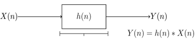
Fig 11 LTI System
Let input signal be x[n]
x[n] = 
The output obtained when we apply input as unit sample sequence for n=k
y[n,k] = h[n,k] = H[ [n-k]]
y[n] = H[x[n]]
= H [  ]
]
But y[n,k] = h[n,k] = H[ [n-k]]
Hence, the output will now be
y[n] = [  ]
]
=  ]
]
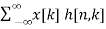
Linear Convolution
Considering an LTI system with input as impulse signal. As we know that impulse response of any system gives complete describes the behavior of any LTI system. Basically, we decompose the input signal first. The apply input as impulse and obtain the corresponding output. Obtained output is then graphically analysed.
Let input signal be x[n]
x[n] = 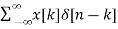
The output obtained when we apply input as unit sample sequence for n=k
y[n,k] = h[n,k] = H[ [n-k]]
Where n= time index
k = location of input impulse parameter
The x[n] because of input weighted sum of output will be
y[n] = H[x[n]]
= H [  ]
]
But y[n,k] = h[n,k] = H[ [n-k]]
Hence, the output will now be
y[n] = [ 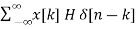 ]
]
=  ] (Due to superposition theorem)
Now, by time invariance property we can write
h[n]= H [
For delayed sequence we have
h[n-k] =H [ ]
]
Hence, the output equation can now be written as
y[n] = [ 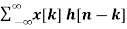 ]
]
The above equation is called as convolution sum.
y[n]= x[n] * h[n]
Example
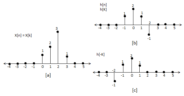
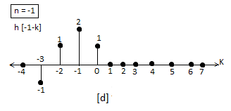
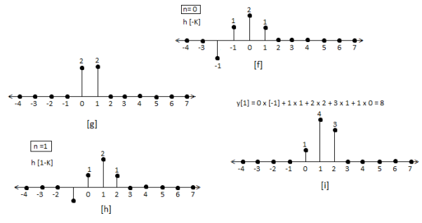
Que) For sequence h[n]={ 1, 2 , 1, -1} determine the response of system with input signal x[n] = {1, 2 ,3 ,1}
Sol:
a) Finding x[k] and h[k] i.e n=k.
b) Folding h[k] we get h[-k].
c) Then shifting the above signal[-k] we get h[1-k]
d) Multiplying above signal h[1-k] with x[n].
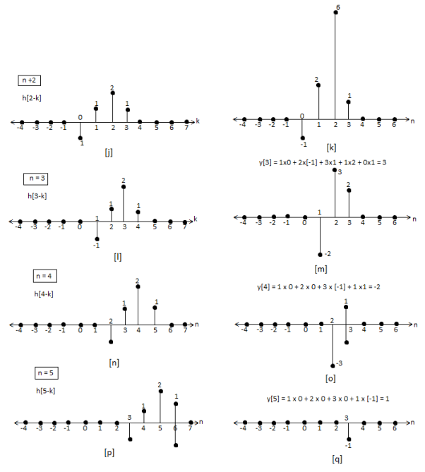
e) Again, incrementing h[1-k] by 1 we get h[2-k] multiplying with x[n].
f) Continuing this process till we get 0 for output y. In this case for n=5.
The graphical representation is shown below.
Convolution by tabulation method
In this method we form a table type structure and find the convolution of x[n] and h[n]. We will understand this by solving an example.
Que) For h[n] = {1, 2, 1, -1}, x[n] = {1, 2, 3, 1}. Find x[n]*h[n]?
Sol:
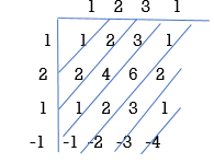
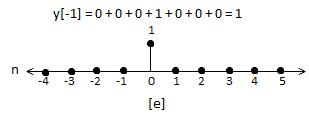
y[-1] = 1
y[0]= 2+2 = 4
y[1] = 1+4+3 = 8
y[2]= -1+2+6+1 = 8
y[3]= -2+3+2 = 3
y[4]= -3+1 = -2
y[5]= -1
y[n]= {1, 4, 8, 8, -2, -1}
The above sequence is the required convolution of x[n] and h[n].
Properties of Linear Convolution
Commutative Law
x(n) * h(n) = h(n) * x(n)


Associate Law
[ x(n) * h1(n) ] * h2(n) = x(n) * [ h1(n) * h2(n) ]


Distribute Law
x(n) * [ h1(n) + h2(n) ] = x(n) * h1(n) + x(n) * h2(n)
Example
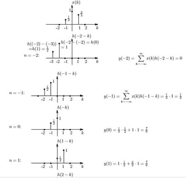
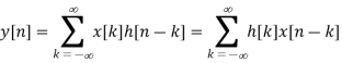
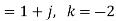
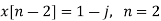
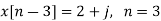
Q1)
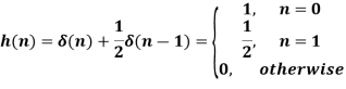
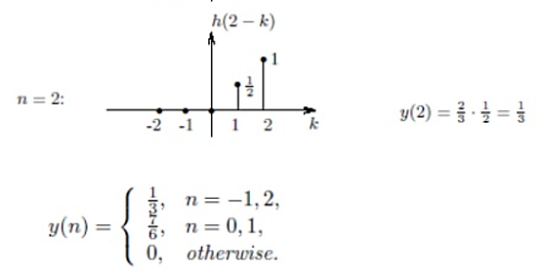
Let us find the response to 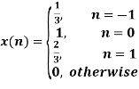 . The impulse response h of the system is the response to the unit impulse:
A1)
(1) flip h;
(2) for a fixed n, shift h by n;
(3) for the same fixed n, multiply x(k) by h(n-k), for each k;
(4) Sum the products over k; 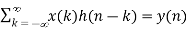
A system is said to be stable if its impulse response satisfies the following criterion
Theorem:
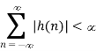
Stability ⟺ 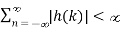 , in the Discrete domain, OR
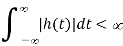
Stability ⟺ 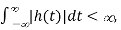 in the continuous domain.
Proof of sufficiency:
Suppose 

We have 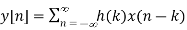
If x[n] is bounded, ie 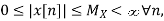 then
then

But as 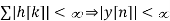
In order for a discrete LTI system to be causal, y[n] must not depend on x[k] for k > n. For this to be true h[n-k]'s corresponding to the x[k]'s for k > n must be zero. This then requires the impulse response of a causal discrete time LTI system satisfy the following conditions:
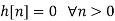
Essentially the system output depends only on the past and the present values of the input
Proof
Let in particular h[k] is not equal to 0, for some k<0.
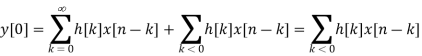
So we need to prove that for all x[n] = 0, n < 0, y[0] = 0
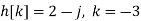
Now we take a signal defined as
This signal is zero elsewhere. Therefore we get the following result:
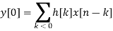
We have come to the result that y[0] 0, for the above assumption. Our assumption stands void. So we conclude that y[n] cannot be independent of x[k] unless h[k] = 0 for k < 0
Sampling usually refers to conversion of continuous signal into short duration of pulses each pulse followed by a skip period when no signal is available. Below shown is a uniformly sampled signal.
Following are two popular sampling operations:
1. Single rate or periodic sampling
2. Multi-rate sampling
Figure below shows the structure and operation of a finite pulse width sampler, where (a) represents the basic block diagram and (b) illustrates the function of the same. T is the sampling period and p is the sample duration.
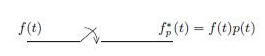
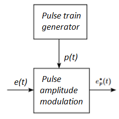
Figure 12(a): Basic block diagram
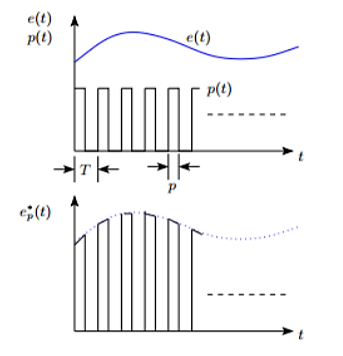
Figure 12(b): Sampler output
Finite pulse width sampler converts a continuous time signal into a pulse modulated or discrete signal. The most common type of modulation in the sampling and hold operation is the pulse amplitude modulation.
The block diagram of sampler is shown above, having a pulse train of p seconds and sampling period of T seconds.
p(t)= unit pulse train with period T
p(t)=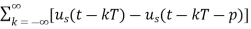
Us(t)=unit step function

In frequency domain p(t) can be represented as
p(t)= 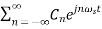
 = 2π/T
Cn=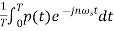
p(t)=1 for 0≤ t ≤p
The output of the ideal sampler can be expressed as
f*(t)=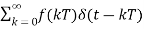
F*(s)=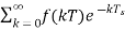
The output of the sampler can be approximated as
Cn=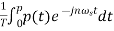
=
In sampling the signal m(t) is multiplied with periodic pulse train. Let M(ω) the spectrum of the input signal be band limited with the maximum frequency of fm as shown in figure 4.
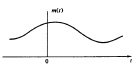
Figure: 13 Spectrum of input signal
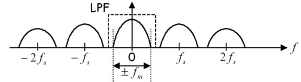
Figure: 14 (fs>2 fm)
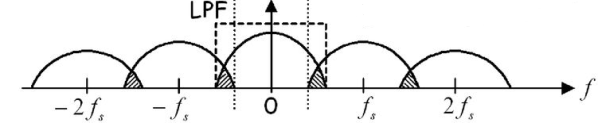
Figure: 15 (fs<2 fm)
The frequency spectrum of this signal when impulse sampled is plotted in figure 5 (for fs>2 fm). In figure 6 for (fs<2 fm). From figure 5 and figure 6 we can conclude that as long as fs≥2fm the original signal is preserved in the sampled signal and can be extracted from it by the low pass filter. This is known as Shannon’s Sampling theorem. This theorem states that the information contained in a signal is fully preserved in the sampled form as long as the sampling frequency is at least twice the maximum frequency contained in the signal.
Sampling in frequency domain is usually used in DFT (Discrete Fourier transform), where continuous signal of spectrum in sampled to get discrete values of spectrum, which results in periodicity in time domain. This helps to process any continuous spectrum signal of non periodic in nature to discretize and digitize for further processing.
The following figure indicates a continuous-time signal x (t) and a sampled signal xs (t). When x (t) is multiplied by a periodic impulse train, the sampled signal xs (t) is obtained.
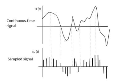
Fig 16 Sampled Signal
Sampling Rate
To discretize the signals, the gap between the samples should be fixed. That gap can be termed as a sampling period Ts.
Sampling Frequency=1/Ts=fs
Where,
- Ts is the sampling time
- Fs is the sampling frequency or the sampling rate
Sampling frequency is the reciprocal of the sampling period. This sampling frequency, can be simply called as Sampling rate. The sampling rate denotes the number of samples taken per second, or for a finite set of values.
Nyquist Rate
Suppose that a signal is band-limited with no frequency components higher than W Hertz. That means, W is the highest frequency. For such a signal, for effective reproduction of the original signal, the sampling rate should be twice the highest frequency.
Which means,
fS=2W
Where,
- fS is the sampling rate
- W is the highest frequency
This rate of sampling is called as Nyquist rate.
Key takeaway
This rate of sampling is called as Nyquist rate.
fS=2W
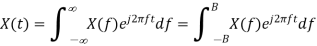
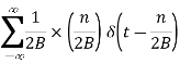
x(t) is Band-limited, with its Fourier transform X(f) being non-zero only in [-B, B]. The dual reasoning of the discussion in previous slide will imply that we can reconstruct X(f) perfectly in [-B, B] by using only the samples x(n / 2B).
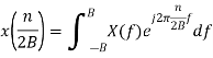
Now
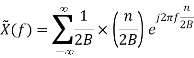
 is the -nth Fourier Series Coefficient
  the periodic extension of X(f).
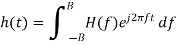
The Fourier inverse of e-j2πto is  (t-to). Therefore, the Fourier inverse
 is
is
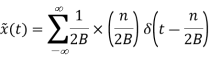
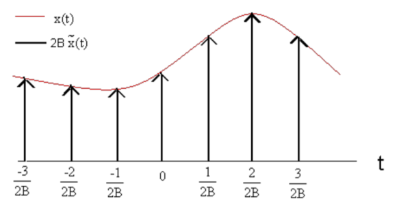
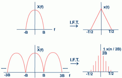
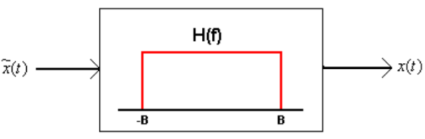
Thus, we see that if we multiply the original Band-limited signal with a periodic train of impulses (period 1/2B, with impulse at the origin of strength 1/2B) we obtain a signal whose Fourier transform is a periodic extension of the original spectrum. We need a mechanism that will blank out the spectrum of  in |f|> B, i.e: multiply the spectrum with:
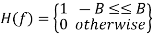
In other words, we need to feed  to an LSI system, the Fourier transform of whose impulse response is the above function (recall the convolution theorem), i.e: one whose impulse response is
Key takeaway
Band-limited signals are infinitely differentiable and very smooth. Given that 'x(t)' is Band-limited with its Fourier transform 'X(f)' being non-zero only in [-B,B] , we can say that
Spectrum that is the periodic extension of 'X(f)' with period 2B
If nature produces analog signals, how do we create digital signals from them? Before we can use digital transmission, we must convert the signal of interest into a digital format. The natural signal (e.g., speech) that we want to transmit will be acquired using an analog device. The analog signal will be translated into a digital signal using a method called analog-to-digital (A/D) conversion. The device used to perform this translation is known as an analog-to-digital converter or ADC. Through A/D conversion, analog signals are changed into a sequence of binary numbers (encoded bits), from which the digital signal is created by the transmitter. This process is depicted below.
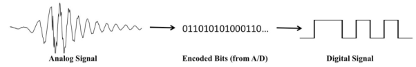
There are two major steps involved in converting an analog signal to a digital signal represented by binary numbers: sampling, and quantizing/encoding.
Steps for A/D conversion:
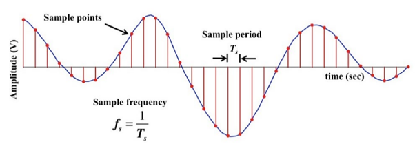
Sampling
This is a process of inspecting the value (voltage) of an analog signal at regular time intervals. The time between samples is referred to as the sample period (T, in seconds), and the number of samples taken per second is referred to as the sample frequency (fs, in samples/second or Hz). Basically, sampling is taking snap-shot values of the analog signal so that you have an accurate representation of how the analog signal is changing over time.
The receiver must convert the bits it receives into sample values, and then recreate what it thinks the analog signal looks like from the samples alone. As you might deduce from the figure below, when the samples are closer together (smaller sample period, which means higher sample frequency), the analog signal is more accurately represented. Note that with the lower sample rates, some of the fluctuations in the analog signal have no samples on them, so the samples are not a good representation of the analog signal.
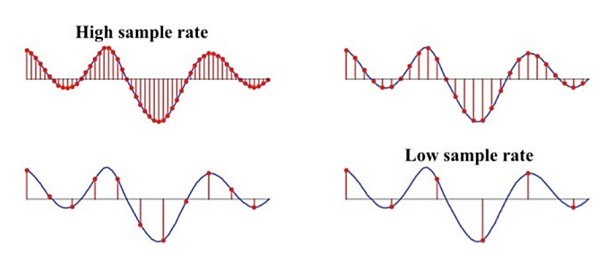
We could consider taking just a few samples (i.e., using a low sampling rate), which means less information to transmit to the receiver. But if we choose that option, when we reconstruct the signal, it will likely be a terrible representation of the original. The low sampling rate will only work well for very slowly changing (low frequency) signals. Alternatively, we could choose the highest possible sampling rate known to man, to ensure that we can accurately capture even very fast signal fluctuations. But the higher the sampling rate, the higher the cost of the equipment and more information must be transmitted. In addition, if we decide to record the communications our saved files will be unnecessarily enormous.
In order to accurately reconstruct an analog signal from its samples, one must sample faster than the Nyquist sampling rate (also called the Nyquist rate), fN, given by the formula
fN= 2fmax
Where fmax is the highest frequency component of the analog signal. That is, the sampling frequency must be more than twice the value of the highest frequency component of the signal:
fs>fN
fN = 2fmax
If the sample rate is not greater than the Nyquist rate, a problem called aliasing results, which can cause severe distortion of your signal.
Quantizing/Encoding
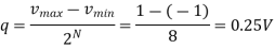
Quantizing/encoding is the process of mapping the sampled analog voltage values to discrete voltage levels, which are then represented by binary numbers (bits). This is needed because the analog sample values are real numbers that occur on a continuum. That is, for example, if a sine wave of amplitude 1V is being sampled, the sample values could be any value between -1V and +1V… an infinite number of possibilities. In any digital system, there is only a finite amount of memory, so only a finite number of values can be used to represent the samples of the analog signal. Converting a sample value from the set of infinite possibilities to one of a finite set of values is called quantization or quantizing. These values are referred to as quantization levels.
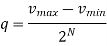
Inputs to A/D converters are limited to a specific voltage range. For the sine wave example above, we assumed that all values of the analog input fall within a range of -1.0 to +1.0 volts (note: this is the typical voltage range of voice or music signals on a computer, such as in .wav or .mp3 files). A/D systems are characterized by the number of bits they have available to perform quantization. The number of bits determines the number of quantization levels. An N-bit A/D converter has 2N quantization levels and outputs binary words of length N (that is, it outputs N-bit values for every sample). For example, a 3-bit A/D system has 23 = 8 quantization levels, so all samples of a 1V analog signal that is input to this A/D will be quantized into one of only 8 possible quantization levels and each sample will be represented by a 3-bit digital word. In general, the A/D converter will partition a range of voltage from some vmin to some vmax into 2N voltage intervals, each of size q volts, where
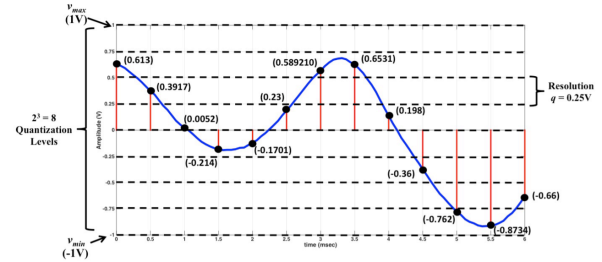
Some common examples of A/D quantizing are digital telephony, which uses 8-bit A/D (28 = 256 quantization levels), CD audio, which uses 16-bit A/D (216 = 65,536 quantization levels), and DVD audio, which uses 24-bit A/D (224 = 16,777,216 quantization levels). The following figures represent conceptually how a 3-bit A/D converter converts an analog signal into bits. In these figures, the analog signal is shown as well as the samples, with samples taken every 0.5 msec (corresponding to a sample rate of fs = 1/0.0005 sec = 2000 samples/sec). The actual analog sample voltages are shown in parentheses next to the samples. Here, the voltage range of the signal is divided into 23 = 8 smaller voltage intervals (also called steps). These are separated by the dashed, bold horizontal lines, and each interval is 0.25V wide:
The value of q is more formally called the quantizer’s resolution.
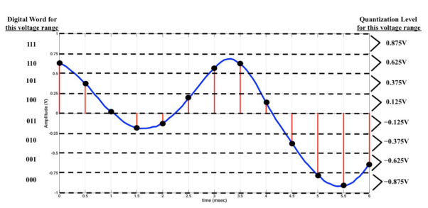
Each of the voltage intervals is assigned an N-bit binary number representing the integers from 0 to 2N-1. For this example, you can see that since we are using a 3-bit A/D, the intervals will be assigned binary numbers representing the integers from 0 to 7 (that is, 000, 001, 010, …, 111), starting from the bottom of the voltage range. In this case, the digital word 000 is assigned to the voltages from -0.75 V to -1.0 V, 001 is assigned to the voltages from -0.5 V to -0.74999 V, and so on. The figure that follows shows for each quantization interval the associated 3-bit digital word (on the left side of the plot). Any analog sample that falls in a given voltage interval will result in those 3 bits being transmitted.
Encoding
When a sample point falls within a given interval, it is assigned the corresponding binary word (this is the Encoding part of Quantization/Encoding). For the first sample point at time 0, the voltage is 0.613 V, which means that sample is assigned a binary value of 110. The A/D then creates a voltage signal that represents these bits, and that process continues as long as an analog signal is input to it. The binary representation of the above signal is:
110 101 100 011 011 100 110 110 100 010 000 000 001.
In this example, every sample produces 3 bits (that is, there are 3 bits/sample). The sample rate was 2000 samples/sec. Multiplying these two values together results in the bit rate (Rb) produced from this A/D conversion:
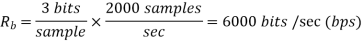
Bitrate is the speed of transfer of data given in number of bits per second. To the right of the plot above is the quantization level associated with each voltage interval. Any analog sample voltage that falls in a given interval is effectively estimated to the center of its quantization level when it is desired to reconstruct the analog signal from the received bits (a receiver may perform this). This process is referred to as Digital-to-Analog conversion (D/A) and will be discussed briefly in the next section. For this example, the quantization level for the lowest voltage interval is the value halfway between -.75 V and -1 V (which is -0.875 V). This means that any analog sample that fell into this range will be represented as -0.875 V.
Key takeaway
Quantizing/encoding is the process of mapping the sampled analog voltage values to discrete voltage levels, which are then represented by binary numbers (bits). This is needed because the analog sample values are real numbers that occur on a continuum
References:
1. Mitra S., “Digital Signal Processing: A Computer Based Approach”, Tata McGraw-Hill,1998, ISBN 0-07-044705-5
2. A.V. Oppenheim, R. W. Schafer, J. R. Buck, “Discrete Time Signal Processing”, 2nd Edition Prentice Hall, ISBN 978-81-317-0492-9
3. Steven W. Smith, “Digital Signal Processing: A Practical Guide for Engineers and Scientists”,1st Edition Elsevier, ISBN: 9780750674447


