UNIT 4
Production analysis
Production function
To have clear knowledge about production and cost it’s mandatory to know the basics of production functions and understand the fundamentals in mathematical terms. We break down short-term and long-term production functions supported variable and glued factors.
What is the production function?
The functional relationship between the physical input (or factor of production) and therefore the output is named a production function. It assumed the input as an explanatory or independent variable and the output as a dependent variable. Mathematically, you can write this as:
Q=f(L,K)
Where"Q"represents the output, "L" and "K" are the inputs, respectively, labour and capital (such as machinery). Note that there may be many other factors, but we are assuming a two-factor input here. Production functions are defined differently in the short term and in the long term. This distinction is crucial in microeconomics. This distinction is based on the nature of the factor input.
Inputs that change directly with the output are called variable factors. These are factors that can change. Fluctuating factors exist both in the short term and in the long term. Examples of variable factors include daily labour and raw materials.
On the other hand, factors that cannot change or change as the output changes are called fixed factors. These factors are usually characteristic only for a short or short period of time. There are no fixed factors in the long term.
Therefore, two production functions can be defined: short-term and long-term. A short-term production function defines the connection between one variable factor (keeping all other factors fixed) and therefore the output. The law of regression to factors explains such a production function.
For example, suppose that a company has 20 units of Labour and 6 acres of land, and initially uses only Labour units (variable coefficients) for that land (fixed coefficients). Thus, the ratio of land and labour is 6: 1. Now, if the company chooses to adopt 2 labour units, then the ratio of land to Labour will be 3: 1 (6: 2).
Here, all factors change in the same proportion. The law used to explain this is called the law of return to scale. It measures how much of the output changes when the input changes proportionally.
|
Key takeaways –
- The functional relationship between the physical input (or factor of production) and therefore the output is named a production function
Total product
Suppose we vary a single input and keep all other inputs constant. Then for different levels of that input, we get different levels of output. This relationship between the variable input and output, keeping all other inputs constant, is often referred to as Total Product (TP) of the variable input.
Average product
Average product is defined as the output per unit of variable input. We calculate it as
APL= TPL / L
Marginal product
Marginal product of an input is defined as the change in output per unit of change in the input when all other inputs are held constant. When capital is held constant, the marginal product of labour is
|

Since inputs cannot take negative values, marginal product is undefined at zero level of input employment. For any level of an input, the sum of marginal products of every proceeding unit of that input gives the total product. So total product is the sum of marginal products.
Labour | TP | MPL | APL |
0 | 0 | – | – |
1 | 10 | 10 | 10 |
2 | 24 | 14 | 12 |
3 | 40 | 16 | 13.33 |
4 | 50 | 10 | 12.5 |
5 | 56 | 6 | 11.2 |
6 | 57 | 1 | 9.5 |
Average product of an input at any degree of employment is the aggregate of all marginal products up to that degree. Average and marginal products are often mentioned to as average and marginal returns, accordingly, to the variable input.
Key takeaways
- Total Product as the total volume or amount of final output produced by a firm using given inputs in a given period of time
- The additional output produced as a result of employing an additional unit of the variable factor input is called the Marginal Product.
- Average product is the output per unit of inputs of variable factors
The law of variable proportion states that keeping all other factors fixed, when the quantity of one factor increased, the marginal product of that factor will eventually decline. This means that upto the use of a certain amount of variable factor, marginal product of the factor may increase and after a certain stage it starts diminishing. When the variable factor becomes relatively abundant, the marginal product may become negative.
Definition
“As the proportion of the factor in a combination of factors is increased after a point, first the marginal and then the average product of that factor will diminish.” Benham
Assumption
The following assumption of law of variable proportion
- The state of technology is assumed to be constant
- Fixed amount of other factors
- The law is based upon the possibility of varying the proportions in which the various factors can be combined to produce a product.
Illustration of the Law:
The law of variable proportion is explained in the below given table and figure. Assume that a there is a given fixed amount of land, in which more labour (variable factor) is used to produce agricultural product.
Units of labour | Total product | Marginal product | Average product |
1 | 2 | 2 | 2 |
2 | 6 | 4 | 3 |
3 | 12 | 6 | 4 |
4 | 16 | 4 | 4 |
5 | 18 | 2 | 3.6 |
6 | 18 | 0 | 3 |
7 | 14 | -4 | 2 |
8 | 8 | -6 | 1 |
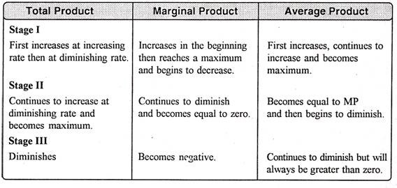
In the above table we can observe that upto the use of 3 units of labour, total product increases at an increasing rate. But after the third unit total product increases at a diminishing rate.
A marginal product is the incremental change in total product as a result of increasing the variable factor i.e labour. We can see from the table, marginal product of labour initially rises and beyond the use of third unit it starts diminishing. The use of 6 units does not add anything in the production. Thus marginal product of labour fallen to zero. After the 6 unit, total product decreases and marginal product becomes negative.
Average product is derived by dividing total product by the quantity of variable unit. Till the 3 unit of labour, average product increases. Whereas after the 3 unit, average product is falling throughout.
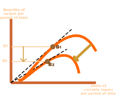
Three Stages of the Law of Variable Proportions:
The stages are discussed in the below figure where labour is measured on the X-axis and output on the Y-axis.
|
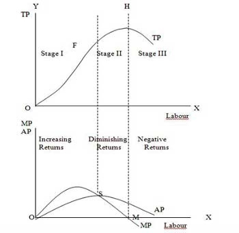
Stage 1. Stage of Increasing Returns:
In this stage, total product increases at an increasing rate till point F..ie the curve TP concave upwards upto point F which means marginal product of labour rises. Because efficiency of fixed factor increases with the increase in variable facto labour. After point F, the total product starts increasing at a diminishing rate. Looking at the next figure, marginal product of labour is maximum, after which it diminishes. This stage is called the stage of increasing returns because the average product of the variable factor labour increases throughout this stage. This stage ends at the point where the average product curve reaches its highest point.
Stage 2. Stage of Diminishing Returns:
The stage 2 ends, when the total product increases at a diminishing rate until it reaches it maximum point H. In this stage both marginal product and average product are diminishing but remain positive. Because fixed factor land becomes inadequate with the increase in the quantity of variable factor labour. At point M marginal product is zero which corresponds to the maximum point H of the total product curve.
Stage 3. Stage of Negative Returns:
In stage 3, with the increase in variable factor labour, the total product decline. Therefore the TP curve slopes downward. As a result, marginal product of labour is negative and MP cure falls below x axis. In this case fixed factor land becomes too much inadequate to the increase in variable factor labour.
|
Key takeaways –
- The law of variable proportion states that keeping all other factors fixed, when the quantity of one factor increased, the marginal product of that factor will eventually decline.
- Three stages are increasing return, diminishing return and negative return
In long run, no factors are fixed. Return of scale refers to proportionate change in productivity from proportionate change in all the inputs.
Definition:
“The term returns to scale refers to the changes in output as all factors change by the same proportion.” Koutsoyiannis
“Returns to scale relates to the behaviour of total output as all inputs are varied and is a long run concept”. Leibhafsky
Types of return of scale
1. Increasing return of scale
2. Constant return of scale
3. Diminishing return of scale
Explanation
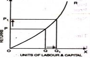
- Increasing return of scale
- When proportionate increase in factors of production leads to higher proportionate increase in production refers to increasing return of scale.
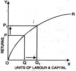
- In the below figure, x axis represent increase in labour and capital while Y axis represent increase in output. When labour and capital increases from Q to Q1, output also increases from P to P1 which is higher than the change in factors of production ie labour and capital
|
2. Diminishing return of scale
- Diminishing return refers to percentage increase in factors of proportion leads to smaller proportion increase in the output
- For instance, 30% increase in variable input (labour and capital) result in 10% increase in output.
- In the below diagram, x axis refers increase in labour and capital while Y axis refers increase in output. Percentage increase in labour and capital from Q to Q1 results in less percentage change in output from P to P1
|
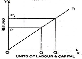
3. Constant return of scale
- Constant return of scale refers to output increases in same proportion in which factors of production (labour and capital) increases.
- Internal and external economies is equal to internal and external diseconomies
- This is known as homogenous production function
- In the below figure, x axis refers increase in labour and capital while Y axis refers increase in output. Increase in labour and capital from Q to Q1 is equal to the increases in output from P To P1
|
Key takeaways –
- Return of scale refers to proportionate change in productivity from proportionate change in all the inputs
Economies of scale are the factors which reduces the production cost as the volume of output increases. This means firm produces more output, then marginal cost of production decreases.
Economies of scale is divided into internal and external
Internal economies of scale – internal economies are caused by factors within the firm. It measures the company efficiency of production. The company focus on improving the output to reduce the product average cost.
Six different types of internal economies of scale: (1) technical, (2) managerial, (3) marketing, (4) financial, (5) commercial, and (6) network economies of scale.
- Technical economies of scale – this can be achieved through improvements and optimizations within the production process. When the output increases, the firm will invest more in efficient equipment and optimise operation based on experience. Efficient machinery result in producing output at lower cost.
2. Managerial economies of scale - The employment of specialised workforce result in managerial economies of scale. As the organisation grow, they hire more expert staff and create a specialised business unit. The firm efficiency is increased by employing specialist, accountants, human resource, etc which will result in reducing the cost of production and increase revenue.
3. Marketing economies of scale – marketing economies of scale is the ability to spread advertising and marketing budget over an increasing output. As the production increases the firm can fix marketing expenses, which will reduce the per unit cost of production. Better advertisement result in reaching larger audience and increase the sale of the firm.
4. Financial economies of scale – access of financial and capital market result in financial economies of scale. Large firms find easier and cheaper to raise funds. As the firm grow, it is considered to be more credit worthy. They can easily raise fund from banks, stock markets.
5. Commercial economies of scale – reduction in price due to discounts or bargaining power result in commercial economies of scale. Larger firms can buy goods and services in larger quantities. Thus they get larger discount and can bargin to negotiate lower prices. This means they pay less for each item purchases.
6. Network economies of scale - when the marginal costs of adding additional customers are extremely low result in network economies of scale. This means larger firm can support large numbers of new customers with their existing infrastructure can substantially increase profitability as they grow.
External economies of scale – external economies of scale are caused by changes outside the firm but within the industry. The factors affect the whole industry. four different types of external economies of scale: (1) infrastructure, (2) supplier, (3) innovation, and (4) lobbying economies of scale.
- Infrastructure - Public infrastructure that is put in place to benefit a specific industry result in infrastructure economies of scale. When many firms of same industry are located nearby, the government will expand infrastructure such as roads, transport, etc to meet their needs.
2. Specialization economies of scale – when suppliers and workers focus on a particular industry due to its size result in specialization economies of scale. When company within the industry increases its size and numbers, suppliers focus in that particular industry. Similarly, similarly workers find job in those industry which is growing in size.
3. Innovation economies of scale – increases public and private research result in innovation economies of scale. Industries have significant impact on the society result in growing public interest. This allows them to collaborate with research facilities and university to improve their products and processes
4. Lobbying economies of scale - Lobbying economies of scale arise from an increase in bargaining power as industries become more significant. The government is ready to compromise as these industry provide a lot of jobs and pay a significant amount of taxes.
Uneconomics of scale occurs when the long-term average cost of an organization increases. It can occur when the tissue becomes excessively large. In other words, uneconomics of Scale Causes larger org-anizations to produce goods and services at increased costs.
There are two types of scale diseconomies: internal diseconomies and external diseconomies, which are discussed as follows:
i.Internal uneconomics of the scale:
See uneconomical raising the cost of production in the organization. The main factors affecting the cost of production of the organization include the lack of determination, supervision and technical difficulties.
ii.External uneconomics of the scale:
See uneconomical to limit the expansion of an organization or industry. Factors acting as restraints on expansion include increased production costs, a shortage of raw materials and a decline in the supply of skilled workers.
There are several causes of diseconomics of scale.
Some of the causes that lead to uneconomics of scale are:
i.Act as the main reason for diseconomics of scale.
If the organization's production goals and objectives are not properly communicated to employees in the organization, they can lead to overproduction or production. This can lead to diseconomics of scale.
Separately, if the communication process in the organization is not strong, then the employee will not get enough feedback. As a result, there will be less face-to-face interaction between employees, which will affect the production process.
ii.Lack of motivation:
This leads to a decrease in productivity levels. For large organizations, workers may feel isolated and less motivated because they are less valued for their work. Because of poor communication networks, it is difficult for employers to interact with employees and build a sense of attributes. This leads to a decrease in the productivity level of output due to lack of motivation. This further leads to an increase in the cost of the organization.
iii.Loss of control:
It serves as the main problem of large organizations. Monitoring and controlling the work of all employees in a large organization becomes impossible and expensive. It is difficult to make sure that all employees of the organization are working towards the same goal. It becomes difficult for managers to direct the sub-coordinates of large organizations.
iv.Cannibalism:
It means a situation where an organization is facing competition from its products. While smaller organizations face competition from the products of other organizations, larger organizations find their products compete with each other.
References
- Business economics by H.L Ahuja
- Business economics application and analysis by Dr. Raj kumar
- Business economics by T Aryamala
- Business economics by SK Agarwal


