UNIT 2
Consumer behavior
In economics utility is the capacity of a commodity to satisfy human wants. Utility of a commodity is its want-satisfying capacity. The more the need of a commodity or the stronger the desire to have it, the greater is the utility derived from the commodity. Utility is subjective. Different individuals can get different levels of utility from the same commodity. For example, someone who likes chocolates will get much higher utility from a chocolate than someone who is not so fond of chocolates
Utility is the basis of consumer demand. A consumer thinks about his demand for a commodity on the basis of utility derived from the commodity.
Definition
According to Prof. Waugh:
“Utility is the power of commodity to satisfy human wants.”
According to Fraser:
“On the whole in recent years the wider definition is preferred and utility is identified, with direness rather than with satisfyingness.”
Types
1. Form Utility:
This utility is created by changing the form or shape of the materials. For example—A cabinet turned out from steel furniture made of wood and so on. Basically, from utility is created by the manufacturing of goods. Form utility can be generated by making use of appropriate design, fine quality materials, and providing a wide range of resources from which to select.
2. Place Utility:
This utility is created by transporting goods from one place to another. Thus, in marketing goods from the factory to the market place, place utility is created. Similarly, when food-grains are shifted from farms to the city market by the grain merchants, place utility is created. Transport services are basically involved in the creation of place utility. In retail trade or distribution services too, place utility is created. Similarly, fisheries and mining also imply the creation of place utility.
3. Time Utility:
Storing, hoarding and preserving certain goods over a period of time may lead to the creation of time utility for such goods e.g., by hoarding or storing food-grains at the time of a bumper harvest and releasing their stocks for sale at the time of scarcity, traders derive the advantage of time utility and thereby fetch higher prices for food-grains. Utility of a commodity is always more at the time of scarcity. Trading essentially involves the creation of time utility.
4. Service Utility:
This utility is created in rendering personal services to the customers by various professionals, such as lawyers, doctors, teachers, bankers, actors etc.
Measures of utility
Cardinal utility
Cardinal utility refers to the proposition that economic prosperity can be rightly perceived and provided with value. Individuals can determine the use of certain products consumed. It prompts measuring of the satisfactory levels in utils.
Ordinal utility
The functions that represent utility of a product according to its preference, but does not provide any numerical figure refers to ordinal utility. Ordinal utility believes that the satisfaction level cannot be evaluated; however, it can be leveled.
Key takeaways
- Utility of a commodity depends on the consumer’s mental attitude and assessment regarding its power to satisfy his particular wants.
- In economics production refers to the creation of utilities in several ways. Its includes form utility, time utility, place utility, service utility.
Law of diminishing marginal utility
The law of diminishing marginal utility describes a familiar and fundamental tendency of human behavior. The law of diminishing marginal utility states that:
“As a consumer consumes more and more units of a specific commodity, the utility from the successive units goes on diminishing”.
Mr. H. Gossen, a German economist, was first to explain this law in 1854. Alfred Marshal later on restated this law in the following words:
“The additional benefit which a person derives from an increase of his stock of a thing diminishes with every increase in the stock that already has”.
This law is based upon three facts
The law of diminishing marginal utility is based upon three facts.
- Total wants of a man are unlimited but each single want can be satisfied. As a man gets more and more units of a commodity, the desire of his for that good goes on falling. A point is reached when the consumer no longer wants any more units of that good.
- Different goods are not perfect substitutes for each other in the satisfaction of various particular wants. As such the marginal utility will decline as the consumer gets additional units of a specific good.
- The marginal utility of money is constant given the consumer’s wealth.
Explanation
Suppose a man is very thirsty. He goes to market and buy a glass of sweet water. The glasses of water give him immense pleasure or say first glass of water is great utility for him. If he takes second glass utility is than first one. If he drinks third glass of water, the utility of the third glass will be less than that of second and so on. And if he increases the glass of water will reach at the stage where he feel negative increase or say utility is declined.
Simply we say in a given span of time the more use of product the lesser will be the utility.
Assumption of the law
Assumptions of law of diminishing utility are:
- Rational behavior of consumer
- Constant marginal utility of money
- Diminishing marginal utility
- Utility is additive
- Consumption to be continuous
- Suitable quantity of a commodity
- Characteristics of the consumer does not change
- No change of fashion, customer, tastes
- No change in the price of commodity
Schedule
Units | Total utility | Marginal utility |
1st glass | 20 | 20 |
2nd glass | 32 | 12 |
3rd glass | 40 | 8 |
4th glass | 42 | 2 |
5th glass | 42 | 0 |
6th glass | 39 | -3 |
From the above table, it is clear that in a given span of time, the first glass of water to a thirsty man gives 20 units of utility. When he takes second glass of water, the marginal utility goes on down to 12 units; When he consumes fifth glass of water, the marginal utility drops down to zero and if the consumption of water is forced further from this point, the utility changes into disutility (-3).
Diagram
|
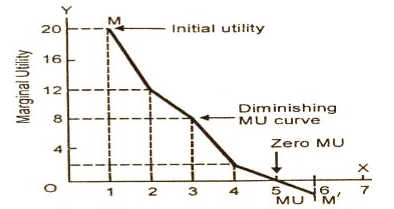
In the above figure, X axis we measure units of a commodity consumed and on the Y axis is shown the marginal utility derived from them. The marginal utility of the first glass of water is called initial utility. It is equal to 20 units. The MU of the 5th glass of water is zero. It is called satiety point. The MU of the 6th glass of water is negative (-3). The MU curve here lies below the OX axis. The utility curve MM/ falls left from left down to the right showing that the marginal utility of the success units of glasses of water is falling.
Law of equi marginal utility
The law of equi-marginal utility is simply an extension of law of diminishing marginal utility to two or more than two commodities. The law of equilibrium utility is known, by various names. It is named as the Law of Substitution, the Law of Maximum Satisfaction, the Law of Indifference, the Proportionate Rule and the Gossen’s Second Law.
In cardinal utility analysis, this law is stated by Lipsey in the following words:
“The household maximizing the utility will so allocate the expenditure between commodities that the utility of the last penny spent on each item is equal”.
The law of equi-marginal utility explains the behaviour of a consumer when he consumers more than one commodity. Wants are unlimited but the income which is available to the consumers to satisfy all his wants is limited. This law explains how the consumer spends his limited income on various commodities to get maximum satisfaction.
Definition
In the words of Prof. Marshall, 'If a person has a thing which can be put to several uses, he will distribute it among these uses in such a way that it has the same marginal utility in all'.
The law states that a consumer should spend his limited income on different commodities in such a way that the last rupee spent on each commodity yield him equal marginal utility in order to get maximum satisfaction.
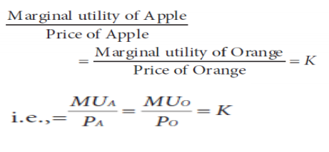
Suppose there are different commodities like A, B, …, N. A consumer will get the maximum satisfaction in the case of equilibrium i.e.,
|

Where MU’s are the marginal utilities for the commodities and P’s are the prices of the commodities.
Assumption
- The consumer is rational so he wants to get maximum satisfaction.
- The utility of each commodity is measurable.
- The marginal utility of money remains constant.
- The income of the consumer is given.
- The prices of the commodities are given.
- The law is based on the law of diminishing marginal utility.
Explanation
Suppose a consumer wants to spend his limited income on Apple and Orange. He is said to be in equilibrium, only when he gets maximum satisfaction with his limited income. Therefore, he will be in equilibrium at the point where the utility derived from the last rupee spent on
|
Law of equi marginal utility schedule
Units | Marginal utility of apple | Marginal utility of orange |
1 | 10 | 8 |
2 | 9 | 7 |
3 | 8 | 6 |
4 | 7 | 5 |
5 | 6 | 4 |
6 | 5 | 3 |
7 | 4 | 2 |
8 | 3 | 1 |
Suppose the ma utility of money is constant at Rs 1 = 5 units, there will buy 6 nits of apple and 5 units of Orange. His total expenditure will be (Rs 5 x 6) + (Rs 4 x 5 ) = Rs 50/- on both commodities. At this point of expenditure his satisfaction is maximized and therefore he will be in equilibrium.
|
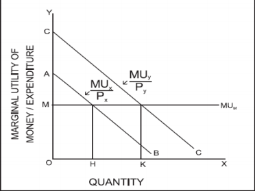
Taking the income of a consumer as given, let his marginal utility of money be constant at OM utils in the above fig. MUX/p X is equal to OM (the marginal utility of money) when OH apple amount of good apple is purchased; MUY/p Y is equal to OM when OK quantity of good orange is purchased. Therefore, the consumer will be in equilibrium when he buys OH of apple and OK of orange.
Limitation
- Invisibility of goods - The theory is weakened by the fact that many commodities like car, house, etc are indivisible. In the case of indivisible goods, the law is not applicable.
- The marginal utility of money is not constant – the theory is based on the assumption that the marginal utility of money is constant. But that is not real so.
- The measurement of utility is not possible – utility is a subjective concept which cannot be measured in quantitative terms.
Key takeaways –
- The law of equi-marginal utility explains the behavior of a consumer when he consumes more than one commodity
- The law of diminishing marginal utility explains an ordinary experience of a consumer. “If a consumer takes more and more units of a same commodity, the additional utility he derives from an extra unit of the commodity goes on falling”
The concept of consumer surplus was originally introduced by classical economists and later modified by Jevons and Jule Dupuit,
Refined form of the concept of consumer surplus was given by Alfred Marshall.
This concept is based on the Law of Diminishing
Definition
“the excess of price which a person would be willing to pay a thing rather than go without the thing, over that which he actually does pay is the economic measure of this surplus satisfaction. This may be called consumer’s surplus”.
Assumption
- The utility can be measured
2. The marginal utilities of money of the consumer remain constant
3. There are no substitutes for the
4. The taste, income and character of the consumer do not change.
5. Utility of one commodity does not depend upon the other commodities
6. Demand for a commodity depends on its price alone; it excludes other determinants of demand
Explanation
Suppose a consumer wants to buy a apple. He is willing to pay 4, but the actual price of the apple is 2. Hence the consumer surplus is 2(4-2).
Therefore, consumer surplus is potential price – actual price
|
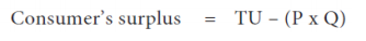
Where,
TU = Total utility
P = price
Q = quantity of the commodity
Consumer surplus schedule
Units of commodity (apple) | Potential price | Actual Price | Consumer surplus |
1 | 6 | 2 | 4 |
2 | 5 | 2 | 3 |
3 | 4 | 2 | 2 |
4 | 3 | 2 | 1 |
5 | 2 | 2 | 0 |
Total | 20 | 10 | 10 |
Diagram
|
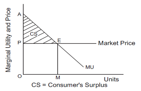
In the above figure, MU is the marginal utility curve. OP is the price and OM is the quantity purchased. For OM units, the consumer is willing to pay OAEM. The actual amount he pays is OPEM. Thus consumer’s surplus is OAEM – OPEM = PAE (the shaded area). A rise in the market price reduces consumer surplus In purchased. A fall in the market price increases the consumer’s surplus.
Criticism
- Utility cannot be measured, because utility is subjective
- Marginal utility of money does not remain constant
- Potential price is internal, it might be known to the consumer himself
Key takeaways –
- The concept of consumer’s surplus is derived from the law of diminishing marginal utility.
- A consumer receives more than he pays for. The excess of benefits from the consumption of a commodity over the sacrifice made in terms of price paid for the commodity is called consumer’s surplus.
Indifference curve analysis
Utility analysis suffers from a flaw in the subjective nature of utility, that is, the inability to measure utility quantitatively and accurately. To overcome this difficulty, economists developed a different approach based on the indifference curve. According to this indifference curve analysis, utility cannot be accurately measured, but the consumer can state which of the combinations of two goods he prefers, without describing the magnitude of the strength of his preference. This means that if the consumer is presented with a number of different combinations of goods, he can order or rank them on a “scale of preference “if the different combinations are marked a, B, C, D, E, etc. In this case, the consumer can tell whether he likes A to B or B to A or is indifferent between them. Similarly, he can show his preference or indifference between other pairs or combinations. The concept of order utility means that consumers cannot go beyond stating their preferences or indifference. In other words, if consumers prefer A to B, they don't know by “how much “they prefer A to B. Consumers cannot state the “quantitative difference “between different satisfaction levels. He can simply compare them “qualitatively". That is, it is possible to determine whether simply one satisfaction is higher than another, or lower, or equal.
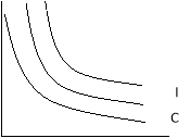
The basic tool of the Hicks-Allen order analysis of demand is the indifference curve, which represents all those combinations of goods that give the consumer the same satisfaction. In other words, all the combinations of goods that lie on the consumer's indifference curve are equally preferred by him. The independence curve is also known as the Iso-utility curve. Indifferent schedules are tabular statements showing different combinations of two goods that bring the same level of satisfaction.
Table Indifference schedule
Combination Rice (X) Wheat (Y)

|
Now consumers are asked to tell the amount of wheat (Y) they are willing to give up the benefit of an additional unit of rice (X) so that the level of satisfaction remains the same. If the profit of one unit of rice fully compensates for the loss of 4 units of wheat, then the following combination of 2 units of rice
And eight units of wheat will give him as much
Satisfaction as the first or first combination. A set of indifferent curves representing the size of preference at different levels of satisfaction are understood because the indifferent curve map (below figure).
Although the combination lying on the indifferent curve 3 (IC3) provides the same satisfaction
Product X
|
Commodity X
Indifference Curve Map
In the above Figure indifference curve map
The level of satisfaction in the indifference curve 3 (IC3) is greater than the level of Satisfaction with indifference curve 2(IC2).
I) the nature of the indifference curve
A) Downward inclination: the indifference curve tilts downwards from left to right.
This means that when the amount of one good in a combination increases, the amount of another must necessarily be reduced so that the total satisfaction is constant.
- If the indifference curve is a horizontal straight line (parallel to the X-axis),
- Then the indifference curve is a horizontal straight line (parallel to the X-axis),
- As shown in the below figure (a) means that as the amount of good X increases,
- The amount of good Y will remain constant, but the consumer will remain
Indifferent among the various combinations.
- This cannot be done, because consumers always prefer
- A large amount of good to a small amount of its good.
- Similarly, the indifference curve cannot be a vertical straight line
(a) Horizontal Fig.2.4 (b) Vertical Fig.2.4(c) Upward Sloping Indifference Curve Indifference Curve Indifference Curve
|


A vertical straight line means that while the amount of good y in combination increases the amount of good X remains constant. The third possibility for the curve is to lean upward to the right.
B) Higher indifference curve gives greater level of utility:
As long as marginal utility of a commodity is positive, an individual will always prefer more of that commodity, as more of the commodity will increase the level of satisfaction.
Combination | Quantity of bananas | Quantity mangoes |
A | 1 | 10 |
B | 2 | 10 |
C | 3 | 10 |
Consider the different combination of bananas and mangoes, A, B and C depicted in table 2.4 and figure 2.7. Combinations A, B and C consist of same quantity of mangoes but different quantities of bananas. Since combination B has more bananas than A, B will provide the individual a higher level of satisfaction than A. Therefore, B will lie on a higher indifference curve than A, depicting higher satisfaction.
Likewise, C has more bananas than B (quantity of mangoes is the same in both B and C). Therefore, C will provide higher level of satisfaction than B, and also lie on a higher indifference curve than B.
|
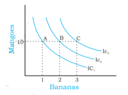
A higher indifference curve consisting of combinations with more of mangoes, or more of bananas, or more of both, will represent combinations that give higher level of satisfaction.
3. Two indifference curves never intersect with each other
Two indifference curves intersecting each other will lead to conflicting results. To explain this, let us allow two indifference curves to intersect each other as shown in the figure 2.8. As points A and B lie on the same indifference curve IC1, utilities derived from combination A and combination B will give the same level of satisfaction. Similarly, as points A and C lie on the same indifference curve IC2, utility derived from combination A and from combination C will give the same level of satisfaction.
|
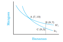
From this, it follows that utility from point B and from point C will also be the same. But this is clearly an absurd result, as on point B, the consumer gets a greater number of mangoes with the same quantity of bananas. So consumer is better off at point B than at point C. Thus, it is clear that intersecting indifference curves will lead to conflicting results. Thus, two indifference curves cannot intersect each other.
Consumer equilibrium
Indifferent map-shows the scale of consumer preferences between various combinations of two goods
Budget line-he shows his money income and various combinations that can afford to buy at the price of both goods.
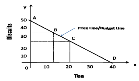
Suppose that the consumer has Rs.20 to spend on tea and biscuits, which cost 50 paise and 40 paise respectively. The consumer has three alternative possibilities before him.
- He may decide to buy tea only, in which case he can buy 40 cups of tea.
- He may decide to buy biscuits only, in which case he can buy 50 biscuits.
- He may decide to buy some quantity of both the goods, say 20 cups of tea (Rs.10) and 25 biscuits (Rs.10) or 12 cups of tea (Rs.6) and 35 biscuits (Rs.14), and so on. (Total amount = Rs.20).
|
The below figure shows the indifference map with 5 indiscriminate curves (ic1, IC2, IC3, IC4, and IC5) and the budget lines PL for good X and good Y. In order to maximize his level of satisfaction, the consumer tries to reach the highest indifference curve. We assume budget constraints, so he will be forced to stay on the budget line.
|
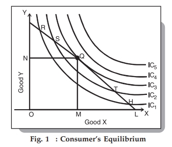
So, what kind of combination is it?
Let's say he chose the combination R from the figure. 1, we see that R is on the low indifference curve–IC1. He can easily afford the combination S, Q, or T that is on a high Ic. Even if he chooses the combination H, the argument is similar because H is on the curve IC1.
Next, let's check out the mixture S lying on the curve IC2. Again, he can reach a better level of satisfaction within the budget by choosing the mixture Q lying on IC3–the argument is analogous for the mixture T, since the higher T is also on the curve IC2.
Therefore, we have left the combination Q.
What happens when he chooses the combination Q?
This is the simplest choice because Q is on his budget line and pts puts him on the simplest possible indifference curve, IC3. There are higher curves, IC4 and IC5, but they are over his budget. Thus, he reaches equilibrium at the point Q on the curve IC3.
Note that at this point the budget line PL is bordered by the indifference curve IC3. Also in this position, consumers buy X in OM amount and Y in ON amount.
Since Point Q is tangent, the slope of line PL and curve IC3 is equal at this point. In addition, the slope of the indifference curve shows that the substitution limit rate (MRSxy) of X with respect to Y is
Hence, at the equilibrium point Q,
MRSxy = MUxMUyMUxMUy = PxPy
Also, the slope of the price line (PL) shows the ratio of X and Y prices. Therefore, we can say that the consumer equilibrium is achieved when the price line is bordered by the indifference curve. Alternatively, when the substitution limit rate of goods X and Y is equal to the ratio between the prices of two goods.
Key takeaways –
- A consumer is in equilibrium when he obtains maximum satisfaction from his expenditure on the commodities he wants to purchase.
- The main theme on the theory of consumer behavior is built is that a consumer attempts to allocate a limited money income among various available goods and services so as to maximise his satisfaction or utility.
References
- Business economics by H.L Ahuja
- Business economics application and analysis by Dr. Raj kumar
- Business economics by T Aryamala
- Business economics by SK Agarwal


