Unit - 5
FIR Filter Design
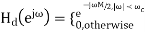
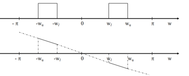
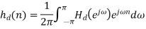
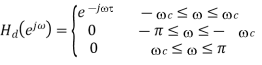
Let the frequency response of the desired LTI ststem we wish to approximate be given by
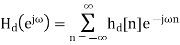
Where  is the corresponding impulse response.
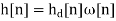
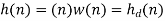
Consider obtaining a casual FIR filter that approximates  by letting
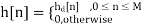
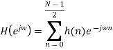
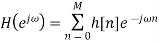
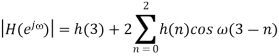
The FIR filter then has frequency response
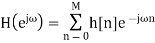
Note that sibce we can write
We are actually forming a finite Fourier series approximation to 
Since the ideal  may contain discontinuities at the band edges, truncation of the Fourier series will result in the Gibbs phenomenon.
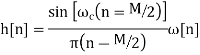
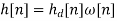
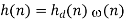
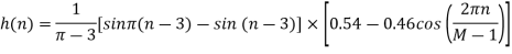
To allow for a less abrupt Fourier series truncation and hence reduce Gibbs phenomenon oscillations, we may generalize h [n] by writing
Where  is a finite duration window function of length M +1.
In practice it may be impossible to use all the terms of a Fourier series. For example, suppose we have a device that manipulates a periodic signal by first finding the Fourier series of the signal, then manipulating the sinusoidal components, and, finally, reconstructing the signal by adding up the modified Fourier series. Such a device will only be able to use a finite number of terms of the series.
Gibbs’ phenomenon occurs near a jump discontinuity in the signal. It says that no matter how many terms you include in your Fourier series there will always be an error in the form of an overshoot near the discontinuity.
The overshoot always be about 9% of the size of the jump. We illustrate with the example. Of the square wave sq(t). The Fourier series of sq(t) fits it well at points of continuity. But there is always an overshoot of about .18 (9% of the jump of 2) near the points of discontinuity.
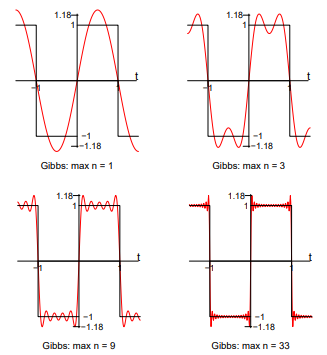
In these figures, for example, ’max n=9’ means we we included the terms for n = 1, 3, 5, 7 and 9 in the Fourier sum
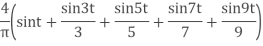
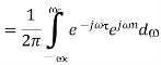
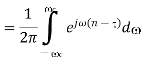
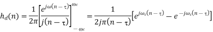
Design an FIR lowpass filter using
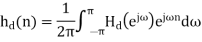
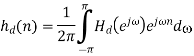
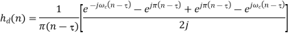
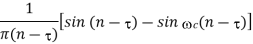
Inverse Fourier transforming we find that
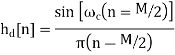
Assuming  is symmetric about M/2, then the linear phaseh[n] is
The relevant lowpass amplitude specifications of interest are shown below
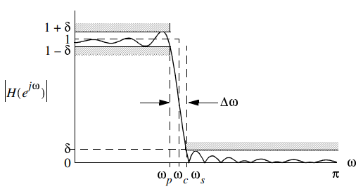
Note that the stop band attenuation in Db is 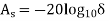 and the peak ripple in Db is
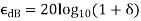
For the Rectangular, Bartlett, Hanning, Hamming and Blackman window functions the relevant design data is given in the following table
Window Characteristic for FIR Filter Design
Window Type | Transition Bandwidth  | Minimum Stopband Attenuation,  | Equivalent Kaiser Window |
Rectangular | 1.81  | 21dB | 0 |
Bartlett |  | 25dB | 1.33 |
Hanning | 5.01  | 44dB | 3.86 |
Hamming |  | 53dB | 4.86 |
Blackman |  | 74dB | 7.04 |
General Design Steps
- Choose the window function
 , that meets the stopband requirements as given in the table above.
 - Choose the filter length M,(actual length is M +1)such that

3. Choose  in the truncated impulse response such that

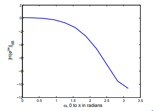
4. Plot  to see if the specifications are satisfied.
5. Adjust  and M if necessary to meet the requirements. If possible reduce M.
Note: this is a “Trial and Error” technique unless one chooses to use a Kaiser window (see below)
Kaiser Window Method
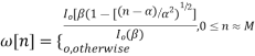
- Let
 be a Kaiser window i.e
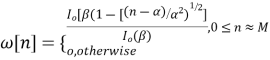
Where 
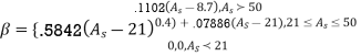
2. Choose  for the specified
  .
.
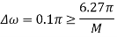
3. The window length M is then chosen to satisfy

4. The value for  is chosen as before
Note: Using the Kaiser empirical formula M can be determined over a wide range of  values to within
  . Very little if any literation is needed.
Design an FIR lowpass using the windowing method such that 
From the window characteristic we immediately see that for  Hammering window will work.
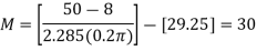
To find M set

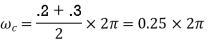
The cutoff frequency is

If a Kaiser window is desired, then for  choose

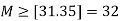
The prescribed value for M should be
Consider a signal that consists of several frequency components passing through a filter.
The phase delay (Tp) of the filter is the amount of time delay each frequency component of the signal suffers in going through the filter.
The group delay (Tg) is the average time delay the composite signal suffers at each frequency.
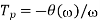
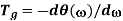
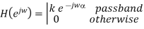
Where Θ(w) is the phase angle
A filter is said to have a linear phase response if,

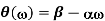
Where α and  are constants
For Example
For ideal LPF
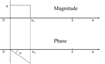
Magnitude response= 
Phase response 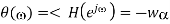
Follows: 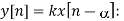 Linear phase implies that the output is a replica of x[n] {LPF} with a time shift of .
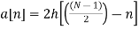
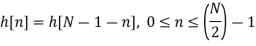
- Symmetric impulse response will yield near phase FIR filters.
Positive symmetry of impulse response
 n=0,1,…,(N-1)/2 (N odd)
N=0,1,…(N/2)-1 (N even)
Negative symmetry of impulse response:
 n=0,1,…,(N-1)/2 (N odd)
n=0,1,…(N/2)-1 (N even)


Types of FIR linear phase systems
1. Type I FIR linear phase system
The impulse response is positive symmetric and N an odd integer.
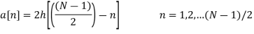
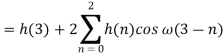
The frequency response is

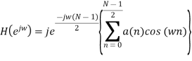
Where 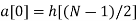
 n=1,2,…,(N-1)/2
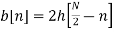
2. Type II FIR linear phase system
The impulse response is positive symmetric and N is an even integer
The frequency response is
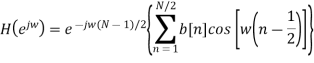
Where

3. Type III FIR linear phase system
The impulse response is negaitve-symmetric and N an odd integer


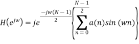
Where
Windowing method
Let the frequency response of the desired LTI ststem we wish to approximate be given by
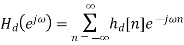
Where  is the corresponding impulse response.
Consider obtaining a casual FIR filter that approximates  by letting
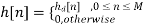
The FIR filter then has frequency response
Note that sibce we can write
We are actually forming a finite Fourier series approximation to 
Since the ideal  may contain discontinuities at the band edges, truncation of the Fourier series will result in the Gibbs phenomenon.
To allow for a less abrupt Fourier series truncation and hence reduce Gibbs phenomenon oscillations, we may generalize h [n] by writing
Where  is a finite duration window function of length M +1.
Filter design using Kaiser window
- Let
 be a Kaiser window i.e
Where 
2. Choose  for the specified
  .
.

3. The window length M is then chosen to satisfy

4. The value for  is chosen as before
Note: Using the Kaiser empirical formula M can be determined over a wide range of  values to within
  . Very little if any literation is needed.
Design an FIR lowpass using the windowing method such that 
From the window characteristic we immediately see that for  Hammering window will work.
To find M set

The cut-off frequency is
If a Kaiser window is desired, then for  choose

The prescribed value for M should be

Rectangular Window
This is the simplest window function but provides the worst performance from the viewpoint of stopband attenuation. The width of main lobe is 4π/N
ωR(n) = 1 for n=0,1,M-1
= 0 otherwise
Magnitude response of rectangular window is
|WR(ω)| = 
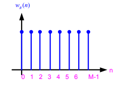
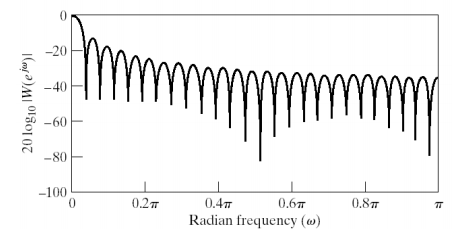
Fig: Rectangular Window
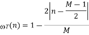
Bartlett (Triangular) Window
Bartlett Window is also Triangular window. The width of main lobe is 8π/M
ωt(n) = 1-
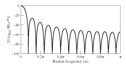
Fig: Bartlett Window
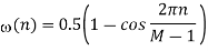
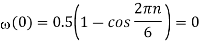
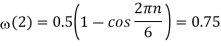
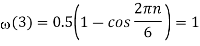
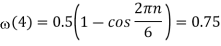
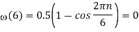
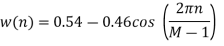
Hanning Window
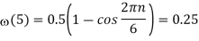
This is a raised cosine window function given by:
W(n) = 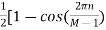 ]
]
W(ω) = 0.5WR(ω) +0.25[WR (ω - ) + WR (ω -
 )]
)]
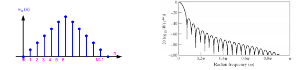
Fig: Hanning Window
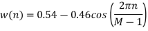
Hamming Window
This is a modified version of the raised cosine window
W(n) = 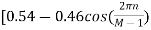 ]
]
W(ω) = 0.54WR(ω) +0.23[WR (ω - ) + WR (ω -
 )]
)]
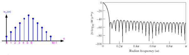
Fig: Hamming Window
Blackman Window
This is a 2nd -order raised cosine window
W(n) = 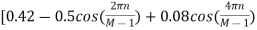 ]
]
W(ω) = 0.42WR(ω) +0.25[WR (ω - ) + WR (ω -
 )]+ 0.04[WR (ω -
 ) + WR (ω -
 )]
)]
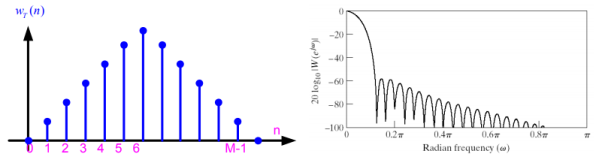
Fig: Blackman Window
Key takeaway
Window name
| Window function |
Rectangular | 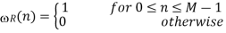 |
Triangular
|  |
Hamming | 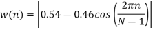 |
Hanning | 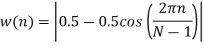 |
Blackman | 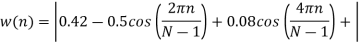 |
Window name | Transition width of main lobe | Min. Stopband attenuation | Peak value of side lobe |
Rectangular |  | -21dB | -21dB |
Hanning |  | -44dB | -31dB |
Hamming |  | -53dB | -41Db |
Barlett |  | -25dB | -25Db |
Blackman |  | -74dB | -57Db |
Example
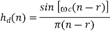
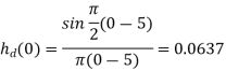
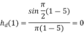
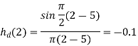
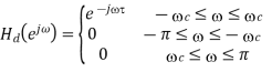
Q1) Design a LPF using rectangular window for the desired frequency response of a low pass filter given by ωc = π/2 rad/sec, and take M=11. Find the values of h(n). Also plot the magnitude response.
Sol:
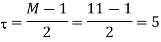
r= M-1/2 = 5
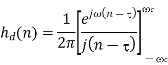
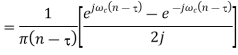
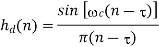
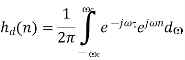
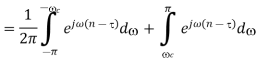
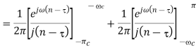
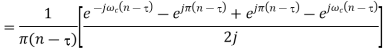
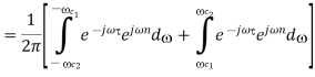
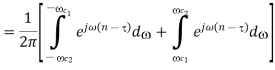
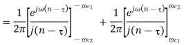
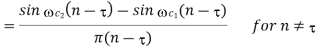
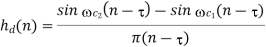
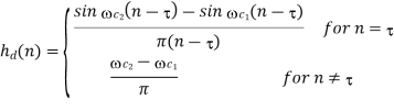
By taking inverse Fourier transform


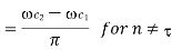
For  and
and 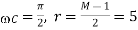
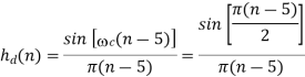
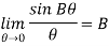
For 
 Using L’Hospital Rule
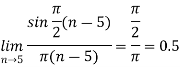
Where 
The given window is rectangular window ω(n) = 1 for 0 ≤ n ≤ 10
=0 Otherwise
This is rectangular window of length M=11. h(n) = hd (n)ω(n) = hd (n) for 0 ≤ n ≤ 10
H[z]=  =
= 
The impulse response is symmetric with M=odd=11


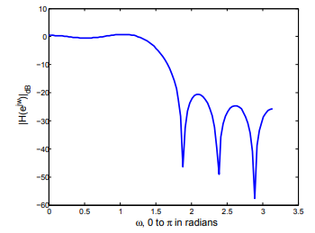
 |  |  |
           |            |            |
Response
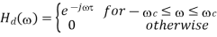
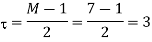
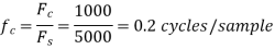
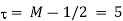
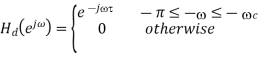
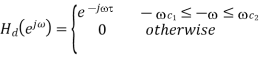
Q2) The desired frequency response of low pass filter is given by Hd (ejω) = e−j3ω − 3π/ 4 ≤ ω ≤ 3π/ 4 and 0 for 3π /4 ≤ |ω| ≤ π Determine the frequency response of the FIR if Hamming window is used with N=7
Sol
t = M-1/2 = 3


For  and
and 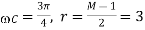
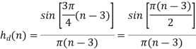
For 
 Using L’Hospital Rule
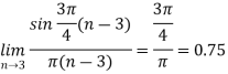
Where 

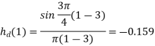
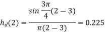
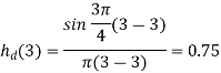
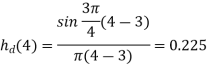

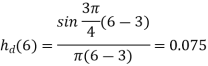
The given window is hamming window
To calculate the value of h(n)


The frequency response is symmetric with M=odd=7


 |  |  |
           |            |        |
RESPONSE
Q3) Design the FIR filter using Hanning window
Sol:

To calculate the value of 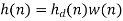


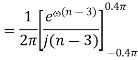
Q4) Design an FIR filter (lowpass) using rectangular window with passband gain of 0 dB, cut-off frequency of 200 Hz, sampling frequency of 1 kHz. Assume the length of the impulse response as 7.
Sol:
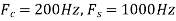
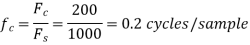


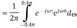
When 
When 
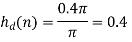
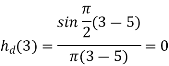
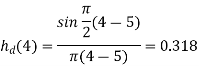
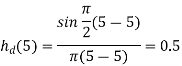
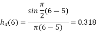
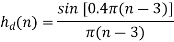
Calculating h(n)
As it is rectangular window h(n) = w(n)=hd(n)=h(n)
For M=7
n |  |
0 | -0.062341 |
1 | 0.093511 |
2 | 0.302609 |
3 | 0.4 |
4 | -0.062341 |
5 | 0.093511 |
6 | 0.302609 |
Q5) Using rectangular window design a lowpass filter with passband gain of unity, cut-off frequency of 1000 Hz, sampling frequency of 5 kHz. The length of the impulse response should be 7.
Sol:
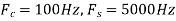


The filter specifications (ωc and M=7) are similar to the previous example. Hence same filter coefficients are obtained.
h (0) =-0.062341, h(1)=0.093511, h(2)=0.302609 h(3)=0.4, h(4)=0.302609, h(5)=0.093511, h(6)=-0.062341
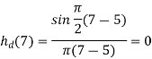
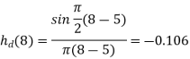
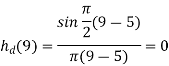
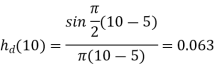
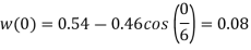
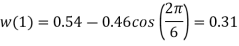
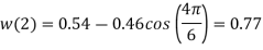
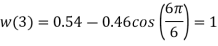
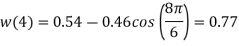
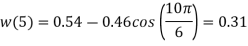
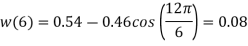
Q6) Design a HPF using Hamming window. Given that cut-off frequency the filter coefficients hd (n) for the desired frequency response of a low pass filter given by ωc = 1rad/sec, and take M=7. Also plot the magnitude response.
Sol:
By taking inverse Fourier transform


The given window function is Hamming window. In this case
 for
for 
 |  |
0 | -0.00119 |
1 | -0.00448 |
2 | -0.2062 |
3 | 0.6816 |
4 | -0.00119 |
5 | -0.00448 |
6 | -0.2062 |
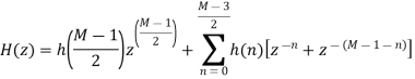
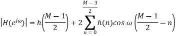
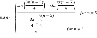
The magnitude response of a symmetric FIR filter with  is
is

For M=7


Q7) Design an ideal bandpass filter having frequency response Hde (jω) for π/ 4 ≤ |ω| ≤ 3π/ 4. Use rectangular window with N=11 in your design.
Sol:

The length of the filter with given is related by
And 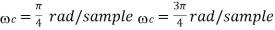
The given window is rectangular hence
For n=0,1,2,…,10 estimate the FIR filter coefficients h(n).
Frequency response of digital filter: 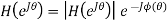
Continuous function of θ with period 2π 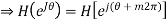
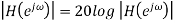
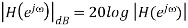
 is the called the Magnitude function.
Magnitude functions are even functions 
 is called the Phase lag) angle
 Phase functions are odd functions
- More convenient to use the magnitude squared and group delay functions than
 and
and 
- Magnitude squared function: 
- It is assumed that H(z) has real coefficients only.
- Group delay function (θ) . Measure of the delay of the filter response.
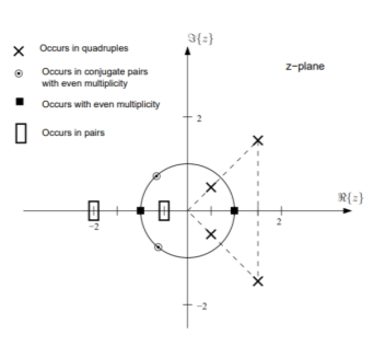
Complex zeros  and poles
  occur in conjugate pairs.
If  is a real zero/pole of
 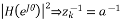 is also a real zero/pole.
If  is a zero/pole of
  are also zeros/poles.
Magnitude and Phase Characteristics
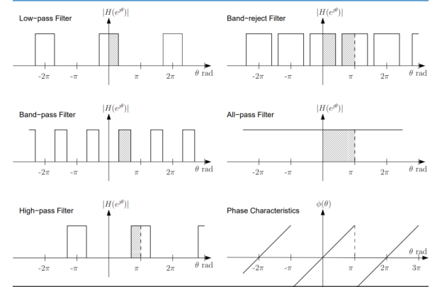
“Linear Phase” refers to the condition where the phase response of the filter is a linear (straight-line) function of frequency (excluding phase wraps at +/- 180 degrees). This results in the delay through the filter being the same at all frequencies. Therefore, the filter does not cause “phase distortion” or “delay distortion”. The lack of phase/delay distortion can be a critical advantage of FIR filters over IIR and analog filters in certain systems, for example, in digital data modems.
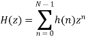
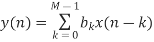
For an N-tap FIR filter with coefficients h(k), whose output is described by:
y(n)=h(0)x(n) + h(1)x(n-1) + h(2)x(n-2) + … h(N-1)x(n-N-1),
The filter’s Z transform is:
H(z)=h(0)z-0 + h(1)z-1 + h(2)z-2 + … h(N-1)z-(N-1) , or
The variable z in H(z) is a continuous complex variable, and we can describe it as: z=r·ejw, where r is a magnitude and w is the angle of z. If we let r=1, then H(z) around the unit circle becomes the filter’s frequency response H(jw). This means that substituting ejw for z in H(z) gives us an expression for the filter’s frequency response H(w), which is:
H(jw)=h(0)e-j0w + h(1)e-j1w + h(2)e-j2w + … h(N-1)e-j(N-1)w , or
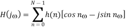
Using Euler’s identity, e-ja=cos(a) – jsin(a), we can write H(w) in rectangular form as:
H(jw)=h(0)[cos(0w) – jsin(0w)] + h(1)[cos(1w) – jsin(1w)] + … h(N-1)[cos((N-1)w) – jsin((N-1)w)] , or
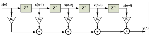
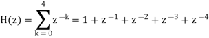
The direct form is obtained from
Based on the above equation, we need the current input sample and M−1 previous samples of the input to produce an output point. For M=5, we can simply obtain the following diagram from Equation 1.
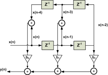
On the other hand, for a linear-phase FIR filter, we observe the following symmetry in coefficients of the difference equation
The structure obtained from the above equation is shown in Figure 2. While Figure 1 requires five multipliers, employing the symmetry of a linear-phase FIR filter, we can implement the filter using only three multipliers. This example shows that for an odd M, the symmetry property reduces the number of multipliers of an (M−1)th-order FIR filter from M to M+1/2.
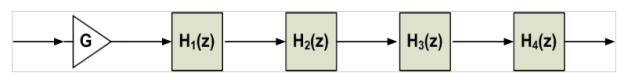
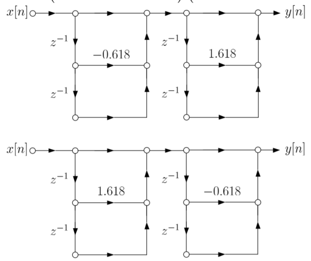
Cascade form
The cascade structure is obtained from the system function H(z). The idea is to decompose the target system function into a cascade of second-order FIR systems. In other words, we need to find second-order systems which satisfy
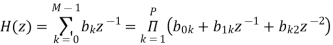
Where P is the integer part of M/2. For example, M=5, H(z) will be a polynomial of degree four which can be decomposed into two second-order sections. Each of these second-order filters can be realized using a direct form structure. It is desirable to set a pair of complex-conjugate roots for each of the second-order sections so that the coefficients become real.
Assume that we need to implement the nine-tap FIR filter given by the following table using a cascade structure.
k | 4 | 3 and 5 | 2 and 6 | 1 and 7 | 0 and 8 |
 | 0.3333 | 0.2813 | 0.1497 | 0 | -0.0977 |
Solution:
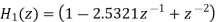
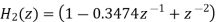
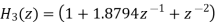
The system function of this filter is

It can be show
Where

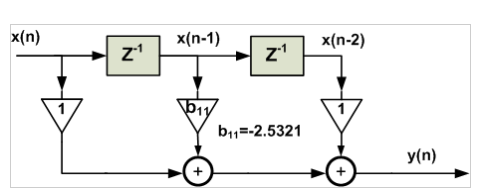
Linear phase structure
The symmetry (or antisymmetry) property of a linear-phase FIR filter can be exploited to reduce the number of multipliers into almost half of that in the direct form implementations • Consider a length-7 Type 1 FIR transfer function with a symmetric impulse response:


We obtain the realization shown below
- A similar decomposition can be applied to a Type 2 FIR transfer function
- For example, a length-8 Type 2 FIR transfer function can be expressed as

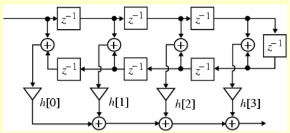
The Type 1 linear-phase structure for a length-7 FIR filter requires 4 multipliers, whereas a direct form realization requires 7 multipliers
Examples
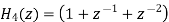
Q) Draw using the cascade form for the LTI system whose transfer function is
A) Hence H(z) can be factorized as

Although it can be realized with first-order sections, complex coefficients are needed, which implies higher computational cost. To guarantee real-valued coefficients, we group the sections of complex conjugates together.


References:
1. Ifeachor E.C, Jervis B. W, “Digital Signal Processing: Practical approach”, Pearson Publication, 2nd Edition.
2. Li Tan, “Digital Signal Processing: Fundamentals and Applications”, Academic Press, 3rd Edition.
3. Schaum's Outline of “Theory and Problems of Digital Signal Processing”, 2nd Edition.
4. Oppenheim, Schafer, “Discrete-time Signal Processing”, Pearson Education, 1st Edition.
5. K.A. Navas, R. Jayadevan, “Lab Primer through MATLAB”, PHI, Eastern Economy Edition.


