Unit - 4
Segments, Illumination models, Color model and Shading
4.1.1 Introduction of Segment
Segment is smallest possible area in two points in computer graphics.
It is in form of array like a table that keeps the commands in a way to display it at the screen.
The segment has following four parts.
- Index
- Size
- Position
- Visibility
The visualization of particular part of picture, sub division of picture done by using segment in computer graphics.
The scaling, rotation and translation of picture perform in the presence on segment.
Each segment is associated with components.
The components consist of set of attributes and image transformation parameters like scaling, rotation.
Following are two types of segment.
- Posted segment
- Un-posted segment
4.1.2 Segment Table
The segment table is used to keep the record of length of similar segments in its memory.
The new entry in the table includes the length of segment.
It is used to check the segment is already in its memory, if exist the bit is ultimately required.
Following figure 4.1.2 shows the segment table.
|
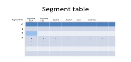
Fig. no. 4.1.2
4.1.3 Segment Creation
The segment is created if no other segment is opened.
Since two segments can’t be opened at the same time as it is difficult to assign the drawing instruction to particular segment.
The segment created must have valid name to identify.
There should not be the same name of two segments.
Following are some steps to create a segment.
- If any other segment is opened then give error and stop.
- If no segment is present then read name of new segment.
- Check the name of segment, if it is not valid then print “not valid”.
- If name is already existing then print error.
- Make new free storage area in display file and start the new segment.
- Initialize the size of new segment to 0 and make all attributes as default.
- Inform new segment is open now.
- Stop
4.1.4 Segment Closing
The segment needs to be closed after all display file instructions then renamed the segment as 0.
If two unnamed segments are present then no need to be delete the segment.
Following are some steps to close the segment:
- If segment is not open then print error.
- Rename the currently open segment as 0.
- Delete other segments that may have been saved and initialize the unnamed segment with no instructions.
- Make the new free storage and start the unnamed segment.
- Initialize the size of unnamed segment to 0.
- Stop
4.1.5 Segment Deleting
The segment should be deleting without destroying the entire display and recover the space occupied by the segment as shown in figure.
|
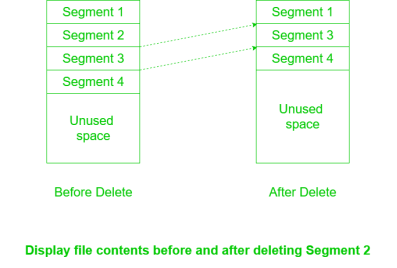
Fig. no. 4.1.5
Following are some step to delete the segment:
- Read the name of segment to be deleted.
- If the segment name is not valid then print error.
- If the segment is open then print error.
- If size of the segment is less than 0 then no processing happens and stop.
- The other segments that follow the deleted segment they will be shifted by their size.
- Reuse the space by resetting the index of next free instruction.
- The starting position of shifted segment is adjusted by subtracting the size of deleted segment from it.
- Stop
4.1.6 Segment Renaming:
The segment renaming is used to achieve double buffering.
Double buffering means the one copy is for showing and other for create, alter and for animation.
Following are some step to rename the segment:
- If both old and new segment names are not valid then print error.
- If any of two segments is open then print error.
- If new segment name is already existing then show error.
- The old segment table is copied into new position.
- Delete the old segment
- Stop
4.1.7 Segment Visibility
Each segment is having the visibility attribute.
The segment’s visibility is stored in an array as part of the segment table.
By checking this array we can determine whether or not the segment should be displayed.
Figure 4.1.7 shows the visibility along line, point and from segment.
|
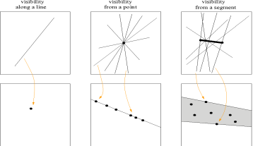
Fig. no. 4.1.7
4.2 Illumination Models
It is also called as lighting model or shading model.
It is used to calculate the intensity of light which is reflected at the given point on surface.
4.2.1 Light Sources
The lighting effects are depend on three factors:
Light source: the light sources can be point source, parallel source, distributed source etc.
Surface: the light falls on the surface part and reflects.
Observer: the position of the observer and the sensor spectrum sensitivities that also effects the light.
Following are the illumination models.
4.2.2 Ambient Light
This also referred to available lighting in an environment.
Suppose the observer is standing on the road facing the building with exterior of glass and the sun rays are falling on building reflecting back from it and falling on the object under observation.
This is known as ambient illumination.
Where the source of light is indirect then it is refered as ambient illumination.
The reflected intensity Iamb =Ka * Ia
Where Ka is the surface ambient reflectivity value which varies from 0 to 1, Ia is the ambient light intensity.
4.2.3 Diffuse light
The diffuse reflection is the reflection of the rays that are scattered in many angles from the surface.
In the specular reflection the ray incident on the surface is scattered at one angle only.
The surface of the reflection should have equal luminance when viewed from all direction lying in the half space adjacent to the surface.
The surface can be plaster or fibers as paper, polycrystalline material.
The surface of reflection in diffuse reflection is rough or grainy.
The light source and the surface made angle that shows the brightness of a point.
The reflected intensity Idiff of a point on the surface:
Idiff = Kd * Ip cos(Ꙫ) = Kd * Ip (N * L)
Where Ip is the point light intensity, Kd is the surface diffuse reflectivity value, N is the surface normal and L is the light direction.
Following figure 4.2 (a) shows the diffuse and specular reflection from the glossy surface.
|
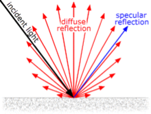
Fig. no. 4.2 (a)
4.2.4 Specular Reflection
It is a regular reflection.
The specular reflection of light reflects from the surface like mirror reflection.
The specular reflection contrasted the diffuse reflection.
In specular reflection the light is scattered from the surface in the range of the direction.
Following figure 4.2 (b) shows the coplanar condition of the specular reflection.
|

Fig. no. 4.2 (b)
4.2.5 Phong Model
It is an empirical model for specular reflection. It is also referred as phong illumination or phong lighting. It is also known as the phong shading in 3D graphics. The formula for the calculation of the reflected intensity I spec. Ispec=W(Ꙫ) I * cos n (ф) Where W(Ꙫ) is Ks, L is the light source, N is the normal surface, R is the direction of reflected ray, V is the direction of observer, Ꙫ be the angle between L and R, ф be the angle between R and V. |
4.2.6 Combined Diffuse and Specular Reflections with Multiple Light Source
For a single point light source, the combined diffuse and the specular reflection from the point on an illuminated surface as, I=Idiff + Ispec = Ka . Ia + Kd . I (N . L) + Kc . I (N . H) If we place the more than one point source then we obtain the light reflection at any surface point by summing the contribution from the individual sources. |
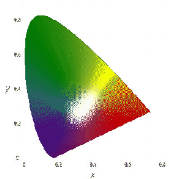
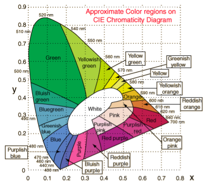
4.3.1 CIE Chromaticity Diagram
CIE stands for Commision Internationale Eclairage. The RGB values become unpleasant when the values of RGB representation are negative. It is defined in 1931 in base terms of virtual primary axes X, Y and Z. This axes are used to allow to match all visible colors as linear combination with positive coefficient only. Hence it is known as the chromaticity values X, Y, Z. The visible colors can be expressed as the C=XX+YY+ZZ. The normalization processed and it becomes X+Y+Z=1. This gives new coordinates as x, y and z =1-x-y which are independent on luminous energy X+Y+Z. The coordinates of visible chromatic value form a horseshoe shaped region with the spectrally pure colors on the curved boundary. Following figure 4.3 (a) shows the horseshoe shape of the visible region.
Fig. no. 4.3 (a)
Following is the figure 4.3 (b) of CIE chromaticity.
Fig. no. 4.3 (b) |
4.3.2 Color Gamut
The color gamut is used to describe the range of color within the spectrum of colors.
This colors are identified by by the human eye i.e. visible color spectrum.
It is a subset of colors used in computer graphics.
The subset of colors are used to represent the given circumstances within given color space.
The output device generally use gamut to sense the original colors which are lost in process.
Following figure 4.3 (c) shows the color Gamut.
|
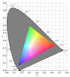
Fig. no. 4.3 (c)
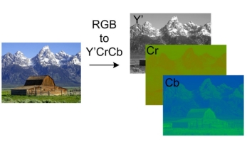
4.3.3 YCbCr
It is used as part of image color. It is used in pipeline video, digital photography systems. It is also reffered as YPb/Cb Pr/Cr, Y’CbCr. Y’ is the luma component and Cb and Cr are the blue ab=nd red difference chroma components. Y’ is difeered by Y i. e. luminance (light intensity is nonlinear based on gamma corrected RGB primaries) This color space can defined by mathematical coordinate transformation from associated RGB colors. Following figure 4.3 (d) shows the representation of RGB to YCbCr transformation.
Fig. no. 4.3 (d) |
4.3.4 RGB
It is color space which is commonly used.
RGB stands for Red Green Blue.
The RGB model states that the image having more colors and that colors are made up of three different images i.e red image, black image and blue image.
The grayscale image is shown by only one matrix but color image is shown by three different matrices.
One color image matrix contains: red matrix + green matrix + blue matrix
Application of RGB
- Liquid crystal display (LCD)
- Plasma display or LED display such as TV
- Cathode ray tube (CRT)
- Compute monitor or large scale screen
4.3.5 HSV
It is also known as HSB (Hue Saturation Brightness)
HSV stands for Hue Saturation Value.
In HSV there are three main components are: Hue, saturation and the value.
It defines the shades and the brightness of the color.
It may be depicted as cone or cylinder.
There are secondary colors In HSV are red, yellow, green, cyan, blue and magenta.
It also having the mixture of adjacent pairs of them.
It is an alternative representation of RGB model.
The colors of each hue are arrange in radial slice.
The slices are placed around the central axis of neutral colors.
This neutral colors are ranges from the black at the bottom to white at the top.
The saturation dimension resembling various tints of brightly colored paint that colors are mix together to represent the HSV color model.
The value dimension resembling the mixture of paint is vary with the amount of black and white color.
The geometric cylinder of HSV starts with red primary at 00 passing through green primary at 120o and blue at 240o , then back to red 360o.
The geometry of central vertical axis comprises neutral, achromatic or gray colors ranging from top to bottom.
The range starts from the white at lightness 1 to black at lightness 0.
Following is the figure 4.3 (e) of HSV.
|
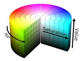
Fig. no. 4.3 (e)
4.3.6 CMY
The CMY color model is a subtractive color model.
The CMY color model named from three colors as Cyan Magenta Yellow.
It contains the cyan, magenta and yellow color.
Thus main colors are used to reproduce various colors of array.
Thus are the primary color but this is not used to specify as absolute because of CMY does not meant by cyan, magenta and yellow mixture.
When the cyan, yellow and magenta becomes exact chromaticity’s of color then it can be specified as absolute color space.
The mixture of subtracted dyes of wavelength from the spectral power distribution of the illuminating light.
The illuminating light which scatters back into the viewer’s eyes and perceives as colors.
Following figure 4.3 (f) shows the CMY color model.
|
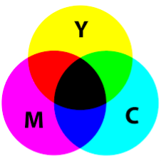
Fig. no. 4.3(f)
It is an implementation of the illumination model at the pixel points or polygon surfaces.
It is used to display colors in graphics and also used to compute the intensities.
It has two important ingredients as properties of the surface and properties of the illumination falling on it.
In intensity computation the object illumination is the most significant thing.
The diffuse illumination is the illumination which has the uniformly reflection from all the direction.
The shading models are used to determine the shade of a point on the surface of an object in terms of number of attributes.
Following figure 4.4 shows the energy comes out from the point on a surface.
|
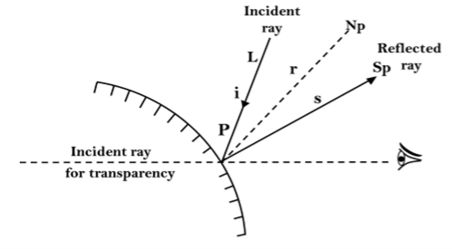
Fig. no. 4.4
4.4.1 Constant Intensity Shading
It is a fast and simple method to render any object with polygon surfaces.
It is also refereed as flat shading.
For each polygon the single intensity is calculated.
All points over the surfaces of the polygon are displayed with the same intensity value.
It is generally used for the quick displaying of curved surfaces.
It consist of illumination model to determine the shade entire polygon according to intensity value.
It is easy to implement.
4.4.2 Halftone Algorithm
It is reprographic shading technique.
It is used to simulate continues tone imagery through dots.
The dots varies in the size or in spacing.
Hence the dots represents the gradient like effect.
Halftone is used to refer the image that is produced by this process.
The range of color in continuous tone goes to infinite or in the range of gray.
It reduces the visual reproduction of the image.
The image that is reducing can be printed with only one color of ink or dot can be differs in size or spacing.
The reproduction relies on the optical illusion.
The halftone dots are so small that human eyes interprets it the patterned areas if they were smooth tones.
Following figure 4.4 (a) shows the halftone dots and human eye interpretation.
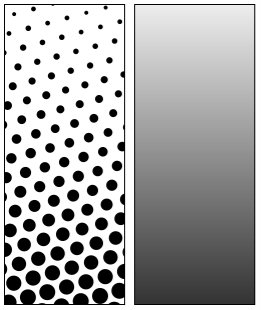
Fig. no. 4.4 (a)
4.4.3 Gourand Algorithm
It is also known as gouraud shading when it renders a polygon surface by linear interpolating intensity value across the surface.
It is an intensity interpolation scheme.
The intensity values for each polygon are coordinates with the value of adjacent polygon along the common edges.
Hence eliminating the intensities discontinuities happens like flat shading.
Following are some calculations that are occurred in gauraud shading.
Determining average unit normal vector at each polygon vertex
Apply an illumination model to each vertex to determine the vertex intensity
Linear interpolate the vertex intensities over the surface of the polygon.
The normal vector obtain by averaging the surface normal of all polygons staring that vertex from each polygon vertex.
Following figure 4.4 (b) shows the Gauraud shading.
|
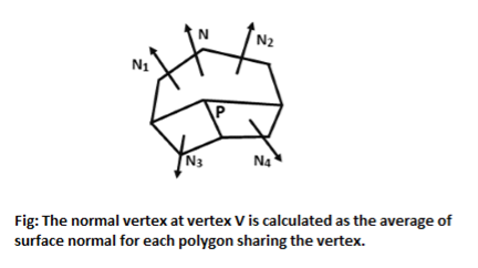
Fig. no. 4.4 (b)
4.4.4 Phong Shading
It is a more accurate method to render a polygon surface.
The polygon surface that interpolates the normal vertex and then apply the illumination model to each surface point.
This method is also known as the normal vector interpolation shading.
It is used to display more realistic highlights on the surface.
It is also use to reduce the match band effect.
Following are the steps to render a polygon surface using phong shading:
- Determining average unit normal vector at each polygon vertex
- Linear and interpolate the vertex normals over the surface of the polygon.
- Apply an illumination model to each scan line to determine the projected intensities for surface points.
Following figure 4.4 (c) shows the phone shading between two vertices.
|
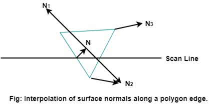
Fig. no. 4.4 (c)
The evaluation of normal between the scam lines are determined by the incremental method along with each scan line.
The illumination model is applied on each of the scan line to determine the surface intensity at that point.
The accurate result is produced by the intensity calculation using approximated normal vector at each point along the scan line instead of using the direct interpolation of intensities.
The phone shading requires more calculations than other shading algorithms.
References
- S. Harrington, “Computer Graphics” ‖, 2nd Edition, McGraw-Hill Publications, 1987, ISBN 0 – 07– 100472 – 6.
- Donald D. Hearn and Baker, “Computer Graphics with OpenGL”, 4th Edition, ISBN-13:9780136053583.
- D. Rogers, “Procedural Elements for Computer Graphics”, 2nd Edition, Tata McGraw-Hill Publication, 2001, ISBN 0 – 07 – 047371 – 4.
- J. Foley, V. Dam, S. Feiner, J. Hughes, “Computer Graphics Principles and Practice” ‖, 2nd Edition, Pearson Education, 2003, ISBN 81 – 7808 – 038 – 9.
- D. Rogers, J. Adams, “Mathematical Elements for Computer Graphics” ‖, 2nd Edition, Tata McGraw Hill Publication, 2002, ISBN 0 – 07 – 048677 – 8.


