Unit 1
INTRODUCTION TO INTERNATIONAL TRADE
International trade theories are simply different theories to elucidate international trade. Trade is the concept of exchanging goods and services between two people or entities. International trade is then the concept of this exchange between people or entities in two different countries.
People or entities trade because they believe that they have the benefit of the exchange. They’ll need or want the products or services. While at the surface, this many sound very simple, there's a good deal of theory, policy, and business strategy that constitutes international trade.
In this section, you’ll study the various trade theories that have evolved over the past century and which are most relevant today. Additionally, you’ll explore the factors that impact international trade and the way businesses and governments use these factors to their respective benefits to promote their interests.
|
David Ricardo agreed that absolute difference in cost gives a clear reason for trade to take place. He, however, went further to argue that even when a country has absolute advantage in the production of both commodities it is beneficial for that country to specialise in the production of that commodity in which it has a greater comparative advantage. The other country can be left to specialise in the production of that commodity in which it has less comparative advantage. According to Ricardo the essence for international trade is not the absolute difference in cost but comparative difference in cost. Ricardian theory is based on the following assumptions.
- Assumptions
- There are two countries and two commodities.
- There is perfect competition both in commodity and factor markets.
- Cost of production is expressed in terms of labour i.e. value of a commodity is measured in terms of labour hours/days required to produce it. Commodities are also exchanged on the basis of labour content of each good.
- Labour is the only factors of production other than natural resources.
- Labour is homogeneous i.e., identical in efficiency, in a particular country.
- Labour is perfectly mobile within a country but perfectly immobile between countries.
- There is free trade i.e., the movement of goods between countries is not hindered by any restrictions.
- Production is subject to constant returns to scale.
- There is no technological change.
- Trade between two countries takes place on barter system.
- Full employment exists in both countries.
- There is no transport cost.
On the basis of the above assumptions, David Ricardo explained his comparative cost difference theory, taking England and Portugal as two countries and wine and cloth as two commodities.
Country | 1 unit of wine | 1 unit of cloth |
England | 120L | 100L |
Portugal | 80L | 90L |
Portugal requires is less hours of labour for both wine and cloth. One unit of wine in Portugal is produced with the help of 80 labour hours as against 120 labour hours required in England. From this it could be argued that there is no need for trade as Portugal produces both commodities at a lower cost. Ricardo however, tried to prove that Portugal stands to gain by specializing in the commodities in which it has a greater comparative advantage. Comparative cost advantage of Portugal can be expressed in terms of cost ratio.
Cost ratios of producing wine and cloth can be expressed as:
Portugal | England | ||
wine | Cloth | wine | cloth |
80/120 < 90/100 | 120/80 > 100/90 | ||
0.66 < 0.9 | 1.5 > 1.11 | ||
Portugal has advantage of lower cost of production both in wine and cloth. However, the difference in cost that is the comparative advantage is greater in the production of wine (1.5-0.66=0.84) than in cloth (1.11-0.9-0.21).
Even in terms of absolute number of days of labour Portugal has a larger comparative advantage in wine, that is, 40 labourers less than England as compared to cloth where the difference is only 10, (40>10). Accordingly, Portugal specializes in the production of cloth where its comparative disadvantage is lesser than in wine.
Comparative Cost Benefits Both: Let us explain Ricardian contention that comparative cost benefits both the participants, though one of them had clear cost advantage in both commodities. To prove it, let us work out the internal exchange ratio.
Country | Wine | Cloth | domestic exchange rate |
| W : C | ||
England Portugal | 120 80 | 100 90 | 1: 1.2 1 : 0.89 |
Let us assume these two countries enter into trade at an international exchange rate (Terms of Trade) 1:1.
At this rate, England specializing in cloth and exporting one unit of cloth gets in turn one unit of wine. At home it is required to give 1.2 units of cloth for unit of wine. England thus gains 0.2 of cloth i.e. wine is cheaper from Portugal by 0.2 unit of cloth.
Similarly, Portugal gets one unit of cloth from England for its one unit of wine as against 0.89 of cloth at home thus gaining extra cloth of 0.11. Here both England and Portugal gain from the trade i.e. England gives 0.2 less of cloth to get one unit of wine and Portugal gets 0.11 more of cloth for one unit of wine.
In this example, Portugal specializes in wine where it has greater comparative advantage leaving cloth at home for England in which it has less comparative disadvantage. The example also validates Ricardian Argument that the base for international trade is the comparative difference in cost and not the absolute difference in cost.
Introduction:
The drawbacks of the classical theory of international trade induced the Swedish economist Prof. Heckscher (1919) to develop an alternate explanation of comparative advantage theory. His theory was further improved by his pupil Bertil Ohlin (1933). Hence it is known as Heckscher-Ohlin (H-O) theory.
Heckscher-Ohlin (H-O) theory argues that there is no need for a separate theory to explain international trade. According to it, international trade is but a special case of interregional trade. Factor immobility which was the base for a separate explanation of international trade by classical economists, does not hold true as factors are mobile or immobile even between two regions of the same country and also between the two countries. It is difference in degree rather than in nature.
The Modern or Heckscher-Ohlin (H-O) Theory explains the new approach to comparative advantage on the basis of general value theory. From all the forces that work together in general equilibrium, H-O theory isolates the differences in physical availability or supply of factors of production among the nations to explain the difference in relative commodity prices and trade between the countries. According to this theory “a nation will export the commodity whose production requires the intensive use of the nation’s relatively abundant and cheap factor and import the commodity whose production requires the intensive use of the nation’s relatively scarce and expensive factor”.
H-O theory explains the modern approach to international theory on the basis of the following assumptions:
- There are two countries, each having two factors (Labour and capital) and producing two commodities.
- There are perfect competitions in both commodity and factor markets.
- All production functions are homogeneous of the first degree i.e. production is subject to constant returns to scale.
- Factors are mobile within the country and immobile between countries. In international trade commodities move between the countries instead of factors.
- The two countries differ in factor supply.
- Each commodity differs in factor intensity.
- Factor intensity differ between the commodities but are same in both countries for each commodity i.e. if goods X is labour intensive, it will be so in both countries. However, goods X and Y differ in factor intensity in the same country.
- Full employment of factor exists in both economies.
- Trade is free i.e. there are no trade restrictions in the form of tariffs or non-tariff barriers.
- No transport cost.
On the basis of the above assumptions it can be stated that (i) each commodity differ in factor intensity (ii) each country differs in factor endowments leading to differences in factor prices. It is therefore necessary to understand the above terms factors intensity and factor abundance in order to explain H-O theory.
(A) Factor Intensity
In our two country commodity model, commodity Y is capital intensive if the capital-labour ratio (K/L) in the production of Y is greater than K/L used in the proportion of X. To explain with an example, if commodity Y requires 2 units of capital (2K) and 2 units of labour (2L), the capital-labour ratio (K/L) for producing commodity Y is 2/2 = 1. For commodity X, if the required inputs are 1K and 4L, the capital-labour (K/L) ratio ¼.
The ratios can be stated as:
For commodity Y, the K/L = 2K /2L = 1
For commodity X, the K/L = 1K/4L =1/4
Here commodity Y is capital intensive and X is labour intensive
Commodity | Capital | Labour | K/L Ratio |
Y X | 2 3 | 2 12 | 1 1/4 |
Capital or labour intensity is not measured in absolute terms but by the ratio i.e. units of capital per labour or units of labour per capital. In our example, K/L ratio for Y is 1 and for X is ¼.
Instead, if units of capital and labour used in the production of Y are 2K and 2L where as for X, 3K and 12L, commodity Y still remains capital intensive through X requires more capital in absolute terms i.e. 3K. capital used per labour in the production of X is 3K/2L i.e. 3/12 = ¼. Where as for Y it is 2K/2L = 1 as shown in table.
Commodity | Capital | Labour | K/L Ratio |
Y X | 2 3 | 2 12 | 1 1/4 |
Factor intensity, therefore is measured by the factor ratios and not by absolute units.
In our example of two commodities, two factors and two countries, we say commodity Y is capital intensive if capital-labour ratio (K/L) of Y is greater than the K/L ratio of X. to illustrate the point let us say that production of one unit of Y requires two units of capital (2K) and 2 unit labour (2L).the capital-labour ratio (K/L) of Y is2/2 =1. Similarly, if the production of X requires 3K and 12L, the capital-labour ratio of X is ¼. Here we say Y is capital intensive and X is labour intensive.
It is to be noted that goods are not categorized based on absolute quantity or units of capital and labour used in the production of a unit of good Y or X but the ratio of capital-labour of each c6K and 24L, here good X requires more capital in absolute number than Y. Yet in terms of ratio, it is Y which is capital intensive (5/5 =1) whereas X is labour intensive (6/24 = ¼).
(B) Factor Abundance
Factor Abundance in Physical Terms
Nations differ in factor endowments. Some have more natural resources, some have more of labour and others more of capital. A given county’s factor abundance can be defined either in physical terms or in terms of relative factor prices. In our two country model, country I is capital abundant, if in physical terms the ratio of total amount of capital (TK) to the total amount of labour (TL) that is (TK/TL) in nation 1 is greater than nation 2 i.e. > . It should be noted that it is not the absolute amount of capital and labour but the ratio of the total amount of capital to the total amount of labour. Country 1 may have a lesser quantity of capital than country 2, yet country 1 will be capital abundant if TK to TL in country 1 is greater than in country 2.
Factor abundance in physical terms can also be explained with the help of production possibility curve OR production frontier, as shown in fig.
In the diagram below, country I is capital abundant, therefore, its production possibility curve is skewed towards Y-axis. Country II is labour abundant, accordingly its production possibility curve is skewed towards X-axis.
Commodity Y is capital intensive.
Commodity X is labour intensive.
|
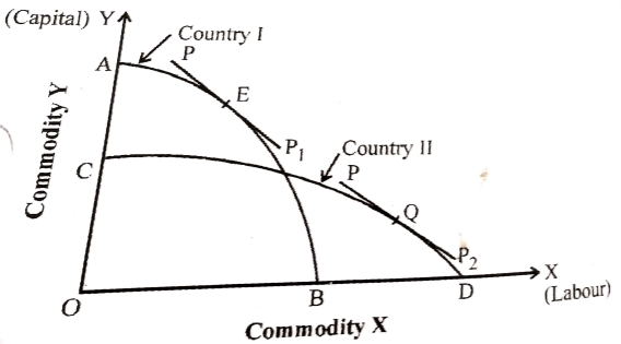
Country I can produce OA of Y i.e. CA quantity more than country II. Similarly, country II can produce OD of X, i.e. BD quantity more than country I. country II can produce more of X which is labour intensive because it is capital intensive due to its abundant capital.
The domestic price lines are PP1 and PP2 in countries I and II. The points E and Q are the respective equilibrium points of production and consumption. The price lines P1 and P2 indicate that commodity Y is cheaper in country I and X in country II, providing the basis for trade.
Factor Abundance in Terms of Factor Price
The cause of international trade is the difference in commodity prices. Price of commodity differs because of cost of production which in turn depends on factor prices. It is therefore necessary to explain factor abundance theory in terms of factor prices.
A nation is capital abundant if the ratio of the capital price to the labour price (PK/PL) is lower in it than in the other.
It can be stated as:
PK1/PL1 < PK2/PL2
The two definitions give us the same meaning. The physical abundance explains the supply side. The price ratios are based on the price of factors determined by the demand for and supply of factors. The demand for factors derived demand i.e. derived from the demand for commodities produced with the help of factors. In our two nations model, demand is assumed to be the same in both the nations. In a country where the supply of physical units of capital (K) is more, its price has to be lower in comparison to the other factor(L). If in nation 1, the price of capital i.e. interest (r) is less than the price of labour i.e. wage (w) and in nation 2, r is more than w, then we have r1/w1 < r2/w2. Here nation 1 is a capital abundant country.
From our above analysis we can derive the following conclusions:
- Each country differs in factors endowments, some have abundant labour, some possess plenty of land and others have huge amount of capital and so on.
- Each country specializes in the production of that commodity which requires more of its abundant factor.
- Abundance of a factor makes it cheaper in terms of its price.
- Low factor prices result in low cost of production and in turn low commodity prices.
- Low commodity price is the basis of international trade.
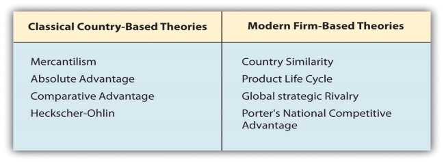
Comparison between Ricardian and Heckscher-Ohlin theories
Ricardian Theory | H.O. (Modern) Theory |
Two Commodities One Factor(Labour) 2-2-1 Model | Two Countries Two Commodities One Factor 2-2-2 Model |
2. Labour is responsible factor for comparative advantage. | Factor abundance is the responsible factor. |
3. Expressed in terms of labour theory. | Expressed in terms of price theory. |
4. International trade requires a separate theory for explanation. | International trade is a special case or extension of inter-regional trade. |
5. Neglects space element. It is one market theory. | Space aspect is considered. It is a multi-market theory |
6. Difference in labour efficiency is taken into account. | Difference in factor supply is taken into account. |
7. Adopted a normative approach concentrating on welfare aspect. | Adopted a positive approach and explained the cause of trade. |
- Net Barter Terms of Trade:
The most widely used concept of the terms of trade is what has been caned the net barker terms of trade which refers to the relation between prices of exports and prices of imports. In symbolic terms:
Tc = Px/Pm
Where,
Tc stands for net barter terms of trade.
Px stands for price of exports (x),
Pm stands for price of imports (m).
When we want to understand the changes in net barter tends of trade over a period of time, we prepare the price index numbers of exports and imports by choosing a particular appropriate base year and acquire the subsequent ratio:
Px1/ Pm1: Px0/ Pm0
. Px„ Pm„
where Px0 and Pm0 represent price index numbers of exports and imports within the base year respectively, and Px1 and Pm1 denote price level numbers of exports and imports respectively within the current year.
Since the costs of both exports and imports within the base year are taken as 100, the terms of trade in the base year would be adequate to one
Px0/ Pm0 = 100/100 = 1
Suppose within the current period the price index number of exports has gone upto 165, and therefore the price index number of imports has risen to 110, then terms of trade in the current period would be:
165/110: 100/100 = 1.5:1
Thus, within the current period, terms of trade have improved by 50 pa’ cent as compared to the base period. Further, it implies that if the prices of exports of a country rise relatively greater than those of its imports, terms of trade for it might improve or become favourable.
On the opposite hand, if the prices of imports rise relatively greater than those of its exports, terms of trade for it might deteriorate or become unfavourable. Thus, net barter terms of trade is a crucial concept which may be applied to measure changes within the capacity of exports of a country to buy the imported products. Obviously, if internet barter terms of trade of a country improve over a period of your time, it can purchase more quantity of imported products for a given volume of its exports.
But the concept of net barter terms of trade suffers from some important limitations therein it shows nothing about the changes within the volume of trade. If the prices of exports rise relatively to those of its imports but because of this rise in prices, the quantity of exports falls substantially, then the gain from rise in export prices could also be offset or maybe more than offset by the decline in exports.
This has been well described by saying, “We make an enormous profit on every sale but we don’t sell much”. so as to overcome this drawback, the net barter terms of trade are weighted by the quantity of exports. This has led to the development of another concept of terms of trade referred to as the income terms of trade which shall be explained later. Even so, internet barter terms of trade is most generally used concept to measure the power of the exports of a country to buy imports.
2. Gross Barter Terms of Trade:
This concept of the gross terms of trade was introduced by F.W. Taussig and in his view this is often an improvement over the concept of net barter terms of trade because it directly takes into account the volume of trade. Accordingly, the gross barter terms of trade ask the relation of the volume of imports to the volume of exports. Thus,
Tg = Qm/Qx
Where
Tg = gross barter terms of trade,
Qm = quantity of imports
Qx = quantity of exports
To compare the change within the trade situation over a period of your time, the subsequent ratio is employed
Qm1/Qx1: Qm0/Qx0
Where the subscript 0 denotes the base year and therefore the subscript I denotes the current year.
It is obvious that the gross barter terms of trade for a country will rise (i.e., will improve) if more imports may be obtained for a given volume of exports. it's important to notice that when the balance of trade is in equilibrium (that is, when value of exports is adequate to the value of imports), the gross barter terms of trade amount to an equivalent thing as net barter terms of trade.
This can be shown as under:
Value of imports = price of imports x quantity of imports = Pm. Qm
Value of exports = Price of exports x quantity of exports = Px. Qx
Therefore, THE balance of trade is in equilibrium.
Px. Qx = Pm. Qm
Px. Qm = Pm Qx
However, when balance of trade is not it equilibrium, the gross barter terms of trade would differ from net barter terms of trade.
Gross barter terms of trade include all the items in the balance of payments thus making its wider and comprehensive than net terms of trade. The gross barter terms of trade differ from the net barter terms of trade as the former include unilateral transfers.
LIMITATIONS
Taussig's concept of gross barter terms of trade has been criticised on the grounds
(a) It expresses the terms of trade in terms of quantity instead of prices. For analytical as well as practical purposes terms of trade expressed in value or price are more relevant.
(b) It includes payments such as unilateral payments which do not depend on trade but on factors mostly unrelated to the trade.
(c) Gross barter terms of trade explain the changes in balance of trade/payments rather than the changes in export-import prices.
(d) A favourable GBTT need not necessarily indicate higher welfare as welfare depends on many factors other than more imports that is favourable GBTT.
3. Income Terms of Trade
In order to enhance upon the net barter terms of trade G.S. Dorrance developed the concept of income terms of trade which is obtained by weighting net barter terms of trade by the volume of exports. Income terms of trade therefore ask the index of the value of exports divided by the price of imports. Symbolically, income terms of trade are often written as
Ty = Px. Qx/Pm
Where
Ty = Income terms of trade
Px = Price of exports
Qx = Volume of exports
Pm= Price of imports
Income terms of trade yields a higher index of the capacity to import of a country and is, indeed, sometimes called ‘capacity to import. this is often because in the long run balance of payments must be in equilibrium the value of exports would be adequate to the value of imports.
Thus, in the long run:
Pm, Qm = Px, Qx
Qm = Px. Qx/Pm
It follows from above that the volume of imports (Qm) which a country can purchase (that is, capacity to import) depends upon the income terms of trade i.e., Px. Qx/Pm. Since income terms of trade may be a better indicator of the capacity to import and since the developing countries are unable to vary Px and Pm. Kindleberger’ thinks it to be superior to the net barter terms of trade for these countries, However, it may be mentioned once more that it's the concept of net barter terms of trade that's usually employed.
The changes in income terms of trade depend on price and volume of exports. An improvement in income terms of trade tells us the increased capacity to import, hence some economist considers it as a better explanation of gains of trade. Other things being equal the capacity to import increases when (i) export prices increase
LIMITATIONS
i) The income terms of trade, however, do not measure precisely the gain or loss from the trade. More imports may be at the cost of higher exports which involve larger amount of domestic resources which could have been used for domestic consumption.
ii) Increase in exports may be due to a decline in prices. With import prices remaining the same, the capacity of the country to import increases. It is, however, possible that additional income is due to increase in exports at a lower price. This
situation, however makes commodity terms of trade deteriorate.
iii) Income terms of trade takes into account the import capacity of a country based on export receipts only but neglects foreign exchange receipts from other sources. It is argued that a country s capacity to import does not depend only on export receipts but on total foreign exchange receipts.
(iv) The concept of income terms of trade fails to consider the welfare aspects of trade. More exports involve more resources to produce those goods. These resources could have been used to produce goods for domestic consumption which have increased the economic welfare of the people.
4. Single Factorial Terms of Trade:
To overcome the limitations of commodity terms of trade, Prof. Viner developed the concept of single factoral terms of trade. This concept admits changes in productivity of factors involved in producing exports. The single factoral terms of trade can be expressed as
Ts = (Px/Pm) Zx
where, Ts = Single factoral terms of trade
Px/Pm= Commodity terms of trade (Tc)
Zx = Productivity index of the export sector
Thus the single factoral terms of trade (Ts) measures the amount of imports the nation gets per unit of domestic factors of production embodied in its exports.
For example, if Tc= 95/110 and the productivity in our export sector rose from 100 in 2015 to 125 in 2019, then our single factoral terms of trade will be
Ts = (95/110) 125 = (0.8636) 125 =107.95
Here the exporting country received 7.95 percent more imports per unit of domestic factors embodied in its exports than what it received in 2015.
LIMITATIONS
i) It is difficult to obtain data to construct a productivity index.
ii) It does not consider the production cost of imports in the import goods producing country.
iii) Comparison between periods becomes impractical as composition of exports and imports may change.
iv) A favourable single factoral terms of trade may lead to a decline in export prices turning Tc of the country unfavorable.
5. Double Factorial Terms of Trade:
To eliminate the drawbacks associated with single factoral terms of trade, Jacob Viner worked out double factoral terms of trade. It can be expressed as:
TD= (Px/Pm) (Zx/Zm) x 100
where, TD= Double factoral terms of trade
Px/ Pm=Tc = Commodity terms of trade
Zx = Export productivity index
Zm=Import productivity index
TD explains the number of units of domestic factors embodied in our exports which are exchanged for a unit of foreign factors embodied in our imports. In other words, it takes into account Improvement in productivity of factors embodied both in export and import goods.
For example,
TD = (95/ 110) (130 / 105) x 100
= (0.8636) (1.2381) x 100=106.92
In this case, the double factoral terms of trade are in favour of their exporting country as its productive efficiency of the factors involved in exports has increased relatively to that of the factors embodied in the imports. In other words, we receive more units of factors of production for a given unit embodied in our exports.
LIMITATION:
i) It is highly difficult to construct the productivity index.
ii) It involves comparison of changes in efficiency in productivity in export and import countries, which is impractical as socio economic and political conditions differ.
iii) Changes in productivity is less important for trading countries than the price and quantity involved in trade.
(iv) Prof. Kindleberger criticised this concept by stating that the exporting country is interested in its gain rather than the improvement in productivity in importing country.
Of all types of terms of trade, only net barter terms of trade, income terms of trade and single factoral terms of trade are made use of for practical purposes. Even from these, it is the net barter terms of trade which are used for all official purposes while measuring terms of trade and changes therein.
6. FACTORS AFFECTING TERMS OF TRADE
Terms of trade of a country are favourable or not, depend on a number of factors. The important of them are:
a) Changes in Factor Endowments: Availability of factors of production in a country may increase or decrease over a period of time. An increase may enable a country to export more and a decrease may lead to increase in imports resulting in changes in terms of trade.
b) Reciprocal Demand: The intensity of demand for other country's goods changes the terms of trade. If India's demand tor goods from China is strong and increasing compared to China's demand for Indian goods, then the terms of trade will be adverse to India.
c) Improvement in Technology: It may lead to reduction in cost of production, requirement of raw materials and other associated changes which may improve the terms of trade. i Developing countries which export raw materials may experience a deterioration in terms of trade due to decline in demand as a result of such changes.
d) Changes in Tastes: Demand for goods may increase or decrease whenever tastes change. Change in taste may include changes in fashion and habits. For example, a change in taste for tea and coffee may affect the terms of trade of those countries which export these items. Declining habit of smoking throughout world may affect the terms of trade of tobacco exporting countries.
e) Tariffs: A country imposes tariffs on its imports to influence its terms of trade in its favour as imports may decline or prices of imports may be reduced by the countries who export these goods.
f) Economic Development: In the process of development an economy experiences dynamic changes leading to the changes in composition and direction of its trade. Besides, changes in quality of inputs, technology and work culture may lead to changes in terms of trade. Some of the developing countries specially emerging market economies are experiencing these changes resulting in positive changes in their terms of trade.
g) Nature of Commodities: The nature and type of goods traded differ from country to country. Developed countries exports mainly comprise capital goods and manufactures. They have a strong demand from the developing countries. Higher cost of production combined with less elastic demand result in high prices for these goods. The developing and poor countries, specially whose exports are mainly primary goods (with some exceptions like crude oil) command less price. The main reasons may be low cost and elastic demand for primary goods. Therefore, it is argued that the developing countries suffer from adverse terms of trade.
As seen above, the share of a country from the gain in international trade depends on the terms of trade. The terms of trade at which the foreign trade would take place is decided by reciprocal demand of every country for the product of the opposite countries.
The theory of reciprocal demand was suggested by JS. Mill and is assumed to be still valid and true even today. By reciprocal demand we mean the relative strength and elasticity of the demand of the two trading countries for each other’s product.
Let us take two countries and B which on the idea of their comparative costs specialize in the production of cloth and wheat respectively. Obviously, country would export cloth to country B, and in exchange import wheat from it. Reciprocal demand means the strength and elasticity of demand of country A for wheat of country B, and therefore the intensity and elasticity of country B’s demand for cloth from country A If the country has inelastic demand for wheat of country B, she is going to be prepared to offer more of cloth for a given amount of wheat. during this case terms of trade are going to be unfavourable thereto and consequently its share of gain from trade are going to be relatively smaller.
On the contrary, if country A’s demand for import of wheat is elastic, it'll be willing to supply a smaller quantity of its cloth for a given quantity of the imports of wheat. During this case terms of trade would be favourable to country A and its share of gain from trade are going to be relatively larger. The equilibrium terms of trade would settle at A level at which its reciprocal demand, that is, quantity of its exports which it'll be willing to offer for a given quantity of its imports is adequate to the reciprocal demand of the opposite country.
Note that the equilibrium terms of trade are determined by the intensity of reciprocal demand of the 2 trading countries but they're going to lie in between the comparative costs (i.e., domestic exchange ratios) of the 2 countries. this is often because no country would be willing to trade at a price which is less than at which it can produce reception.
Let us return to the instance of the 2 countries A and B which specialize in the production of two commodities cloth and wheat respectively, and exchange them with one another.
Production conditions in the two countries are given below:
Table: Production of 1 man per week
|

It will be seen from above table that before trade production conditions in country B are such 12 bushels of wheat would be exchanged for 20 yards of cloth, in it, that is, the domestic exchange ratio is 12: 20 (or 3: 5). On the opposite hand, in country A production conditions are such 4 bushels of wheat would be exchanged for 12, yards of cloth, that is, the domestic exchange ratio is 4: 12 or 1: 3. Obviously, after trade, terms of trade are going to be settled within these domestic exchange ratios of the 2 countries.
The domestic exchange ratios of the 2 countries set the bounds beyond which terms of trade wouldn't settle after trade. it's evident that country B are going to be unwilling to supply more than 12 bushels of wheat for 20 yards of cloth since by sacrificing 12 bushels of wheat it can produce 20 yards of cloth at home.
Likewise, country A wouldn't accept but 6.66 bushels of wheat for 20 yards of cloth, for this is often the domestic exchange rate cloth of wheat for(l :3) determined by production or cost conditions reception in country A.
It is within these limits that terms of trade are going to be settled between the 2 countries as determined by the strength of reciprocal demand of the trading countries. It also follows that it's not mere demand but also the comparative production costs (i.e., the supply conditions) that attend determine the terms of trade. Indeed, the law of reciprocal demand, if properly understood, considers both the forces of demand and supply as determinants of the terms of trade.
Assumptions:
- Two countries
- Two commodities
- Production is subject to constant returns to scale
- No transport cost
- Markets operate under perfect competition
- Existence of full employment
- Free trade between the countries
- Trade is based on comparative cost difference
The theory of reciprocal demand has been explained graphically with the assistance of the concept of offer curves developed by Edgeworth and Marshall. The offer curve of a country shows the amounts of a commodity it offers at various prices for a given quantity of the commodity produced by the opposite country.
To understand how offer curves are derived and the way with their help determination of the terms of trade is explained, we shall first explain how a country reaches its equilibrium position about the amounts of goods to be produced and consumed.
For this purpose, modern economists usually employ the tools of production possibility curve and therefore the community indifference curves. the production possibility curve represents the combinations of two commodities which a country, given its resources and technology, can produce.
A community indifference curve shows the combinations of two goods which give same satisfaction to the community as an entire . A map of community indifference curves portrays the tastes and demand pattern of a community for the 2 goods. A production possibility curve TT’ and a set of community indifference curves IC1IC2 and IC3 of country A are drawn in Fig. 45.1.
The country reaches its equilibrium position with reference to production and consumption of cloth and wheat at the purpose Q where the assembly possibility curve TT’ is tangent to the highest possible indifference curve IC2 at which marginal rate of transformation of fabric for wheat (MRTCW) equals marginal rate of substitution of cloth for wheat (MRSCW) also because the price ratio of the 2 commodities Pc/Pw as shown by the slope of the price line P1P1.
|
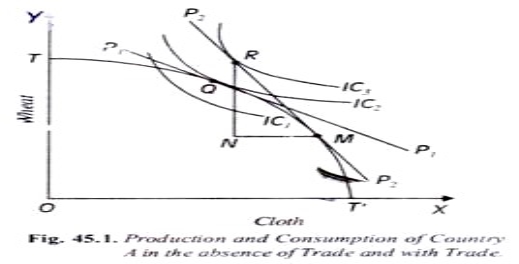
Thus, tangency point Q in Fig. 45.1 depicts the equilibrium position of country within the absence of trade. Suppose country A enters into trade relation with country B and price of cloth rises relative to wheat in order that new price-ratio line becomes P2P2.
It will be observed from Fig. 45.1 that with price- ratio line P2P2 production equilibrium of country is at point M, its consumption equilibrium is at point R. This shows that with price-ratio line PP2 country A will offer or export MN of cloth for RN imports of wheat.
Similarly, if price of cloth further rises relative to wheat, price-ratio line will become more steep, then for an equivalent quantity offered of export of cloth, the or import of wheat will increase. With such information gathered from Fig. 45.1, we are able to derive offer curve of country A in Fig. 45.2.
The tangent line in Fig. 45.1 shows the domestic price ratio of the 2 commodities and features a negative slope. within the analysis of the offer curve, the price line is drawn with a positive slope from the origin. this is because in the drawing of an offer curve we have an interest only in knowing the quantity of 1 commodity which may be exchanged for a particular quantity of another commodity.
In other words, within the analysis of terms of trade what we are really interested is that the absolute slope of the curve, i.e., the price ratio. In Fig. 45.2 the positively sloping price line OP1 from the origin, which in absolute terms, has an equivalent slope as P1P1 of Fig. 45.1 has been drawn. In Fig. 45.2 at price ratio line O1P1 no trade occurs.
When price of cloth rises and price ratio line shifts to OP2 as will be from Fig. 45.2, country A offers ON1 of cloth (exports) for RN1 of wheat (imports). (Note that at a given price ratio what proportion quantity of a commodity, a country will offer for imports from the opposite country is decided by production possibility curve and community’s indifference curves as illustrated in Fig. 45.1).
Suppose the worth of cloth further rises relatively to that of wheat causing the price line to shift to the position OP3. it'll be seen that with the price line OP3, country A is willing to offer for export ON2 quantity of cloth for SN2 of wheat.
|

Likewise, Fig. 45.2 portrays the exports and imports of the country A as price of cloth in terms of wheat increases further and consequently price line shifts further above to OP4 and OP and the new offers of export of cloth for import of wheat are determined by equilibrium points T and U. If points like R, S, T and U representing the country A’s offers of cloth for wheat are joined we get its offer curve.
It is important to notice that the offer curve could also be regarded as the supply curve within the international trade because it shows amounts of cloth which the country A is willing to supply for certain amounts of imports of wheat at various price ratios.
Another important point to be noted is that the offer curve cannot go below the price line OP, which represents the domestic exchange ratio determined by the tangency point Q of production possibility curve and community indifference curve of country A as shown in Fig. 45.1. This is often because, as stated above, no country will be willing to export its product for the quantity of the imported product which is smaller than that it can produce reception.
Likewise, we will derive the offer curve of country B. Figure 45.3 portrays the derivation of the offer curve of country B. representing quantities of wheat which it's willing to exchange for certain quantities of cloth from country A at various prices.
|

Note that so long as country B is importing a smaller quantity of cloth, it'll be willing to supply relatively more wheat for cloth. But because the quantity of imported cloth is increased, it might be prepared to supply relatively less wheat for the given quantity of imports of cloth.
In Fig. 45.3 who’s Y-axis represents wheat, the origin for indifference curves of country B are going to be the North-West Comer Price lines. OP7, OP6, OP5, OP4 etc. express higher price ratios of wheat for cloth. Price line OP1 represents the domestic price ratio in country B within the absence of trade. The points C, D, E, F, G which has been obtained from the equilibrium or tangency points between the community indifference curves of country B and therefore the various price-ratio lines show the equilibrium offers of wheat by country B for cloth of country A at various prices. By joining together points, C. D, E, F and G we obtain the offer curve of country B indicating its demand for cloth of country A in terms of its own product wheat.
|

It would be observed from Fig. 45.2 and 45.3 that offer curves OA and OB of the 2 countries are drawn with an equivalent origin O (i.e., South-West Corner) as the basis. These offer curves represent reciprocal demand of the 2 countries for every other’s product in terms of their own product. The offer curves OA and OB of the 2 countries are brought together in Fig. 45.4. The intersection of the offer curves of the 2 countries determines the equilibrium terms of trade. it'll be seen from Fig. 45.4 that the offer curves of two countries cross at point T. By joining point T with the origin we get the price-ratio line OT whose slope represents the equilibrium terms of trade which can be finally settled between the 2 countries.
At the opposite price-ratio line the offer of a product by country A in exchange for the product of the opposite wouldn't be adequate to the reciprocal offer and demand of the other country B. as an example, at price-ratio line OP1, country B would offer OM wheat for MH or ON of cloth from country A (H lies on B’s offer curve corresponding to price-ratio line OP5).
But at this price-ratio line OP country A would demand much greater quantity of wheat UW for OU of fabric as determined by point W at which the offer curve of country A intersects the price ratio line OP. this may result in rise in price of wheat and therefore the price-ratio line will shift to the right until it reaches the equilibrium position OT or OP4.
On the opposite hand, if price ratio line lies to the right of Or (for instance, if it's OP,), then, as are going to be observed from Fig. 45.4, it cuts the offer curve of country A at point L implying thereby that the country A would offer OR of cloth in exchange for RL of wheat. However, with terms of trade implied by the price ratio line OP4, the country B would demand OZ of cloth for ZS quantity of wheat as determined by point S.
It therefore follows that only at the terms of trade implied by the price ratio line OT (i.e., OP4) that the offer of a product by one country are going to be equal to its demand by the opposite. We therefore conclude that the intersection of the offer curves of the 2 countries determines the equilibrium terms of trade.
As explained above, the offer curves of the 2 countries are determined by their reciprocal demand. Any change within the strength and elasticity of reciprocal demand would cause a change within the offer curves and hence within the equilibrium terms of trade.
It is worthwhile to notice that terms of trade must settle within the price lines OP1 and OP7 representing the domestic rates of exchange between the 2 commodities within the two countries respectively as determined on the idea of production cost and s demand conditions existing in them.
When the terms of trade are settled within these limits set by these price lines OP1 and OP7, both countries would gain from trade, though one may gain relatively more than the opposite depending on the position of terms of trade line.
As explained above, the terms of trade cannot settle beyond these domestic prices ratio lines because just in case of terms of trade line lying beyond these price lines, it'll be advantageous for a country to produce both the products (wheat and cloth) domestically instead of entering into foreign trade.
The various countries of the world have imposed tariffs (i.e., import duties) to protect their domestic industries. it's been said in favour of tariffs that through them a country can provide not only protection to its industries but under appropriate circumstances it also can improve its terms of trade, that is, tariffs under favourable circumstances enable a country to get its imports cheaper.
These favorable circumstances are:
(1) The demand for the exports of the tariff-imposing countries is both large and inelastic
(2) The demand for the imports by the country is sort of elastic. Under these circumstances, as a results of the imposition of tariff by that country, the imports of the country will decline since the worth of the imported commodity will rise. But this is often not the end of the story.
The decline in imports of the tariff-imposing country would reduce the export earnings of its trading partner because it will cause the decrease in demand for it exported commodity. The decrease in demand for the exported commodity within the trading partner would end in lowering its domestic price.
As results of the fall in the domestic price of the exported commodity and so as to maintain its export earnings the exporting country is likely to reduce the price of its exports. this suggests that the tariff- imposing country would now be ready to get its imports at a comparatively cheaper price than before.
Given the demand and price of its exports, the fall in its prices of imports of the tariff- imposing country would imply the improvement in its terms of trade. it's worth mentioning that the improvement in the terms of trade through tariff depends upon the changes in price and resultant changes in quantity demanded of imports and exports of the trading countries which in turn depends upon the elasticity’s of their reciprocal demand.
|
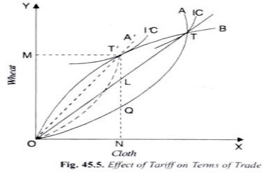
The effects of tariff on the terms of trade are often explained through the geometrical device of offer curves. In Fig. 45.5 the offer curves OA and OB respectively of the 2 countries A and B are shown. These offer curves intersect at T implying thereby that terms of trade adequate to the slope of OT are determined between them.
Now, suppose that country A imposes import duty on wheat from country B. As a results of this imposition of tariff, the offer curve of country A will shift to a new position OA ‘(dotted). this suggests, as an example , that, before tariff, country was prepared to supply ON of fabric for NQ of wheat, but after imposition of tariff it requires NT’ of wheat for ON of cloth and collects QT ‘ as import duty.
It will be noticed from Fig. 45.5 that the new offer curve OA ‘(dotted) of country A intersects the offer curve OB of country B at point T and thereby the terms of trade changes from OT to OT’. Note that the slope of the terms of trade line OT’ is greater than that of OT’.
Thus terms of trade for country A have improved consequent upon the imposition of tariff by country A. as an example , whereas consistent with terms of trade line OT country A was exchanging ON of cloth for N L imports of wheat, it's now exchanging ON of cloth for NT’ of wheat.
The following three things are worth nothing about the impact of tariffs on terms of trade:
1. The gain in terms of trade from imposing a tariff depends on the elasticity of the offer curve of the other trading country. If the offer curve of the other trading country is perfectly elastic, that is, when it's constant costs so that offer curve is that the straight line OB from the origin with slope adequate to that of OT as shown in Fig. 45.6, the imposition of tariff would scale back the quantity of trade between them, the terms of trade remaining the same.
For example, if within the situation depicted in Fig. 45.6 country A imposes a tariff on imports of a wheat from the country B and as a result the offer curve of A shifts upward to the new position OA’ (dotted), the terms of trade remain constant as measured by the slope of the terms of trade line OT. it'll be seen from Fig. 45.6 that in this case only volume of trade has declined from ON to OM
|

2. The gain in terms of trade from imposing a tariff will finally accrue to a country only within the absence of retaliation from the trading country B. But when one country can play a game to improve its position, the opposite can retaliate and play a similar game.
That is, on country A imposing a tariff on its imports from country B during a bid to improve its terms of trade, the latter can even impose a tariff on the imports from the former and thereby cancels out the initial gain by country A. Such competition in imposing tariffs on each other’s product would greatly reduce the volume of trade and leave the terms of trade between them unchanged.
As a result of the reduction in volume of trade, both countries would suffer a loss. “The imposition of tariffs to enhance the terms of trade, followed by retaliation, ensures that both countries lose. The reciprocal removal of tariffs, on the opposite hand, will enable both countries to gain. That’s why different countries enter into bilateral agreements to reduce tariffs on each other’s products.” Further, there's now World Trade Organisation (WTO) which requires the member countries to scale back tariffs so that the volume of international trade expands.
A. Gains from Terms of Trade
The terms of trade refer to the exchange ratio of export and import of goods or their price ratio. It is the ratio of prices of a country’s exports and its imports. The terms of trade determine the gain from trade. On the other hand, an increase in import prices and a stationary or declining export prices will worsen the terms of trade and accordingly the gains from trade too.
Let us discuss the relationship between terms of trade and grains from trade with the following example shown in table.
In our table we express the cost in terms of labour. To produce any particular commodity cost remains the same in a given country but not the same between different countries. In our example, 10 days labour can produce machines or 1 units of cloth in USA but only 2 machines and 8 units of cloth in India.
Labour | Country | Machines | Cloth | Domestic Exchange Rate | |
|
|
|
| Machines | Cloth |
10 days Labour | USA | 10 | 10 | 1 | 1 |
10 days Labour | India | 2 | 8 | 1 | 1 |
Let us suppose that the international exchange rate is 1 unit of machine for 2 units of cloth (1M: 2C). At this rate both countries gain, as U.S.A gets 2C against 1M instead of 1C against 1M that it gets at home. Similarly, India saves 2 units of cloth, since it gets 1 machine by giving 2C against 4C within the country. At the rate 1M: 3.5C, USA’s gain is 2.5C.If the terms of trade settle at 1M: 1.5C, India’s gain in terms of cloth saved its maximum or price paid in terms of cloth is very low.
The gain from trade is maximum if the international terms of trade prevailing are nearer to the country’s internal terms of trade. If the international terms of trade are, for example1:15 which is nearer to the internal terms of trade of USA, then India’s gain is maximum. If they are somewhere nearer to India’s internal terms of trade, say 1:35 USA will gain the most. Thus, the gains from trade are measured with the help of terms of trade.
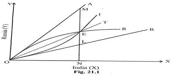
B. Offer Curves- Terms of Trade – Gains From Trade
Economists Alfred Marshall and Francis Edgeworth presented the terms of trade and gains from trade with the help of offer curves. The concept of offer curves is based on J.S Mills reciprocals demand which explains mutual demand for each other country’s commodity in exchange for various quantities of imports at a succession of possible terms of trade.
In diagram 21.1 we have India’s offer curve OI and Russia’s offer curve OR. The diagram explains the domestic rate of exchange the domestic rate of exchange, international terms of trade and gains from trade.
|
C. Increase in World Production
Each country specializes in the production of those commodities for which it is better suited in terms of cost of production. If a country attempts to produce everything what it requires then it may do so at a higher cost and lower production. International trade which is based on international division of labour leads to more production due to international trade with the help of table no 21.2.
Country | Inputs Labour days | Production in Units | Total Output | |
|
| Cloth | Machines |
|
India | 10 | 20 | 4 | 24 |
USA | 10 | 20 | 20 | 40 |
TOTAL |
| 40 | 24 | 64 |
The total production of both countries is 40 cloth and 24 machines, a sum total of 64 units. India, as we can see has a comparative advantage in the production of cloth and USA in machines. If they go for complete specialization applying the labour for producing only one commodity, then India will produce 40 units of cloth and USA 40 units of machines, a sum total of 80 units.
India - 4o units of cloth
USA - 40 units of machines
Total - 80 units
D. Increase in Consumption
With the increase in production as discussed earlier, the increase in consumption of the people of the countries which participate in international trade would also increase. Such positive changes enhance the economic welfare of the people. International trade begins in cheaper and a variety of new goods. Without trade a country will have limited domestic produced goods, that too at a higher price. Internal contact also brings a change in lifestyle. A positive effect of international demonstration effect will result in increased income and consumption.
E. Higher Economic Welfare
International trade, results in increased production due to specialization. As discussed earlier, trade results in additional production and consumption, cheaper and varieties of goods and services resulting in an increase in level of economic welfare. Trade also generates more jobs hence more income. Trade acts as ‘engine of growth’ bringing in all the benefits of growth. All these benefits make people better-off with trade than without.
F. Dynamic Gains
The gains that we discussed so far accrue to the trading countries in a given or static economic situation. There are many other gains which are termed as dynamic gains since the economies undergo changes in terms of technology, production function and finally an outward shift in the that simulates innovation. New ways of producing and organizing production are spread to the local economy through trade and the competitive force of trade simulates adoption of cost-saving techniques. Trade also makes possible economical production of many goods that would otherwise be prohibitive locally.
Reference-
1. Business Economics P.N Chopra
2. Business Economics by H.L Ahuja


