Unit - 5
Finite word length effects in digital filters
Digital Computers use a Binary number system to represent all types of information inside the computers. Alphanumeric characters are represented using binary bits (i.e., 0 and 1). Digital representations are easier to design, storage is easy, accuracy and precision are greater.
There are various types of number representation techniques for digital number representation, for example, Binary number system, octal number system, decimal number system, and hexadecimal number system, etc. But the Binary number system is most relevant and popular for representing numbers in the digital computer system.
Storing Real Number
These are structures as below −
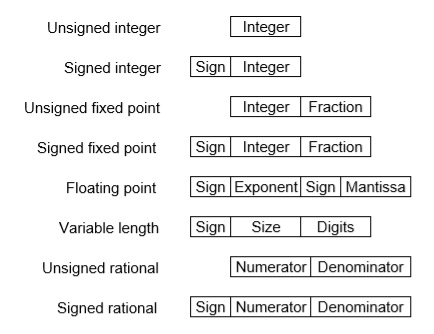
There are two major approaches to store real numbers (i.e., numbers with fractional component) in modern computing. These are (i) Fixed-Point Notation and (ii) Floating Point Notation. In fixed-point notation, there are a fixed number of digits after the decimal point, whereas a floating-point number allows for a varying number of digits after the decimal point.
Fixed-Point Representation −
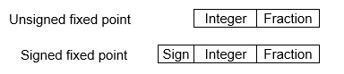
This representation has a fixed number of bits for the integer part and fractional part. For example, if given fixed-point representation is IIII. FFFF, then you can store the minimum value is 0000. 0001 and the maximum value is 9999. 9999. There are three parts of a fixed-point number representation: the sign field, integer field, and fractional field.
We can represent these numbers using:
- Signed representation: range from -(2(k-1)-1) to (2(k-1)-1), for k bits.
- 1’s complement representation: range from -(2(k-1)-1) to (2(k-1)-1), for k bits.
- 2’s complementation representation: range from -(2(k-1)) to (2(k-1)-1), for k bits.
2’s complementation representation is preferred in the computer system because of its unambiguous property and easier of arithmetic operations.
Example −Assume number is using a 32-bit format which reserves 1 bit for the sign, 15 bits for the integer part, and 16 bits for the fractional part.
Then, -43. 625 is represented as follows:
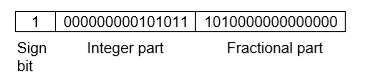
Where 0 is used to represent + and 1 is used to represent. 000000000101011 is a 15-bit binary value for decimal 43 and 1010000000000000 is a 16-bit binary value for fractional 0. 625.
The advantage of using a fixed-point representation is performance and the disadvantage is a relatively limited range of values that they can represent. So, it is usually inadequate for numerical analysis as it does not allow enough numbers and accuracy. A number whose representation exceeds 32 bits would have to be stored inexactly.
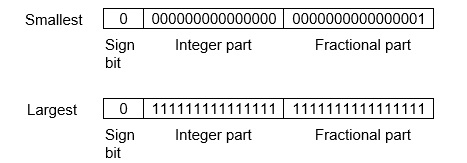
These are above the smallest positive number and largest positive number which can be store in 32-bit representation as given above format. Therefore, the smallest positive number is 2-16 ≈ 0. 000015 approximate and the largest positive number is (215-1) +(1-2-16) =215(1-2-16) =32768, and the gap between these numbers is 2-16.
We can move the radix point either left or right with the help of only integer field is 1.
Floating-Point Representation −
This representation does not reserve a specific number of bits for the integer part or the fractional part. Instead, it reserves a certain number of bits for the number (called the mantissa or significand) and a certain number of bits to say where within that number the decimal place sits (called the exponent).
The floating number representation of a number has two-part: the first part represents a signed fixed-point number called the mantissa. The second part of designates the position of the decimal (or binary) point and is called the exponent. The fixed-point mantissa may be a fraction of an integer. Floating -point is always interpreted to represent a number in the following form: Mxre.
Only the mantissa m and the exponent e are physically represented in the register (including their sign). A floating-point binary number is represented similarly except that it uses base 2 for the exponent. A floating-point number is said to be normalized if the most significant digit of the mantissa is 1.
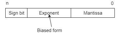
So, the actual number is (-1) s(1+m) x2(e-Bias), where s is the sign bit, m is the mantissa, e is the exponent value, and Bias is the bias number.
Note that signed integers and exponents are represented by either sign representation, or one’s complement representation, or two’s complement representation.
The floating-point representation is more flexible. Any non-zero number can be represented in the normalized form of ± (1. b1b2b3 . . . )2x2n This is the normalized form of a number x.
Example −Suppose the number is using the 32-bit format: the 1-bit sign bit, 8 bits for the signed exponent, and 23 bits for the fractional part. The leading bit 1 is not stored (as it is always 1 for a normalized number) and is referred to as a “hidden bit”.
Then −53.5 is normalized as -53.5= (-110101.1)2= (-1.101011) x25, which is represented as below,
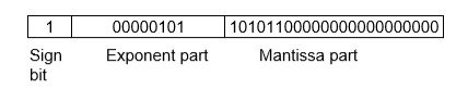
Where 00000101 is the 8-bit binary value of exponent value +5.
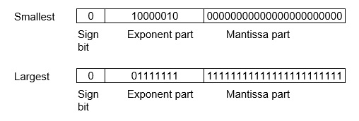
Note that 8-bit exponent field is used to store integer exponents -126 ≤ n ≤ 127.
The smallest normalized positive number that fits into 32 bits is (1. 00000000000000000000000)2x2-126=2-126≈1.18x10-38 and the largest normalized positive number that fits into 32 bits is (1. 11111111111111111111111)2x2127= (224-1) x2104 ≈ 3.40x1038. These numbers are represented as below,
The precision of a floating-point format is the number of positions reserved for binary digits plus one (for the hidden bit). In the examples considered here, the precision is 23+1=24.
The gap between 1 and the next normalized floating-point number is known as machine epsilon. The gap is (1+2-23)-1=2-23for the above example, but this is the same as the smallest positive floating-point number because of non-uniform spacing unlike in the fixed-point scenario.
Note that non-terminating binary numbers can be represented in floating-point representation, e. g., 1/3 = (0. 010101 . . . )2 cannot be a floating-point number as its binary representation is non-terminating.
IEEE Floating point Number Representation −
IEEE (Institute of Electrical and Electronics Engineers) has standardized Floating-Point Representation as the following diagram.
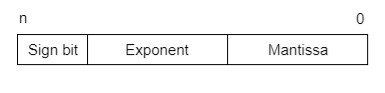
So, the actual number is (-1) s(1+m) x2(e-Bias), where s is the sign bit, m is the mantissa, e is the exponent value, and Bias is the bias number. The sign bit is 0 for a positive number and 1 for a negative number. Exponents are represented by or two’s complement representation.
According to IEEE 754 standard, the floating-point number is represented in the following ways:
- Half Precision (16 bit): 1 sign bit, 5-bit exponent, and 10-bit mantissa
- Single Precision (32 bit): 1 sign bit, 8-bit exponent, and 23-bit mantissa
- Double Precision (64 bit): 1 sign bit, 11-bit exponent, and 52-bit mantissa
- Quadruple Precision (128 bit): 1 sign bit, 15-bit exponent, and 112-bit mantissa
Special Value Representation −
Some special values depended upon different values of the exponent and mantissa in the IEEE 754 standard.
- All the exponent bits 0 with all mantissa bits 0 represents 0. If the sign bit is 0, then +0, else -0.
- All the exponent bits 1 with all mantissa bits 0 represents infinity. If the sign bit is 0, then +∞, else -∞.
- All the exponent bits 0 and mantissa bits non-zero represents a denormalized number.
- All the exponent bits 1 and mantissa bits non-zero represents error.
Key takeaway
Digital Computers use a Binary number system to represent all types of information inside the computers. Alphanumeric characters are represented using binary bits (i.e., 0 and 1). Digital representations are easier to design, storage is easy, accuracy and precision are greater.
There are various types of number representation techniques for digital number representation, for example, Binary number system, octal number system, decimal number system, and hexadecimal number system, etc. But the Binary number system is most relevant and popular for representing numbers in the digital computer system.
The main difference between fixed point and floating point is that the fixed point has a specific number of digits reserved for the integer part and fractional part while the floating point does not have a specific number of digits reserved for the integer part and fractional part.
Fixed point and floating point are two ways of representing numbers. In fixed point, there is a specific number of digits to represent the integer section and fraction section. In other words, there is a fixed number of digits for each portion even though the number is very large or small. On the other hand, in floating point, there is no specific number of digits to represent integer section and fraction section. Floating point representation can cover a large range or numbers when compared to fixed point.
Key takeaway
S.No | Fixed point arithmetic | Float point arithmetic |
1. | Fast operation | Slow operation |
2. | Relatively economical | More expensive because of costlier hardware. |
3. | Small dynamic range | Increased dynamic range. |
4. | Round off errors occurs only for addition | Round off errors can occur with addition and multiplication |
5 | Overflow occur in addition | Overflow does not arise |
6 | Used in small computers | Used in large general purpose computers. |
Quantization noise is a model of quantization error introduced by quantization in the analog-to-digital conversion (ADC). It is a rounding error between the analog input voltage to the ADC and the output digitized value. The noise is non-linear and signal-dependent.
There are two types of Quantization - Uniform Quantization and Non-uniform Quantization.
The type of quantization in which the quantization levels are uniformly spaced is termed as a Uniform Quantization. The type of quantization in which the quantization levels are unequal and mostly the relation between them is logarithmic, is termed as a Non-uniform Quantization.
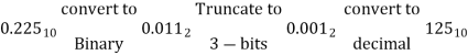
The abrupt termination of given number having a large string of bits (or) Truncation is a process of discarding all bits less significant than the LSB that is retained. Suppose if we truncate the following binary number from 8 bits to 4 bits, we obtain
0.00110011 to 0.0011 (8 bits) (4 bits)
1.01001001 to 1.0100 (8 bits) (4 bits)
When we truncate the number, the signal value is approximated by the highest quantization level that is not greater than the signal.
Truncation error in sign magnitude form:
Consider a 5 bit number which has value of 0.110012 (0.7815)10
This 5 bit number is truncated to a 4 bit number
0.11002 (0.75)10
i.e. 5 bit number 0.11001 has ‘1’ bits
4 bit number 0.1100 has ‘b’ bits
Truncation error, et = 0.1100 – 0.11001
= -0.00001 (-0.03125)10
Here original length is ‘1’ bits. (1=5). The truncated length is ‘b’ bits.
The truncation error, et = 2-b -2-l = -(2-l-2-b)
et = -(2-5 -2-4) = -2-1
The truncation error for a positive number is –(2-b-2-l) ≤et≤0 Non causal
The truncation error for a negative number is 0 et (2-b-2-l) Causal
Truncation error in two’s complement:
- For a positive number, the truncation results in a smaller number and hence remains same as in the case of sign magnitude form.
- For a negative number, the truncation produces negative error in two’s complement –(2-b-2-l) ≤et≤ (2-b-2-l)
Rounding is a quantization method where we ’round-up’ a particular number to the desired number of bits.
Basically, rounding is the process of reducing the size of a binary number to some desirable finite size. This is done in such a way that the rounded off number is as close to the original unquantized number as possible.
Interestingly, the rounding process is a combination of truncation and addition.
In rounding a number to say b-bits, first, the number is truncated to the desired number of bits. Then depending on the number that existed next to the LSB before truncation, an addition to the LSB is performed.
If that particular number (previously next to the LSB) was 0, then 0 is added to the LSB. If that number was 1, then a 1 is added to the LSB.
Consider the same example as above, suppose we wish to truncate the following 8-bit number to 4-bits.
X = 0.01101011 truncates to X = 0.0110
Since the number next to the current LSB was 1, we add 1 to the current LSB.
Thus X is now 0.0111
Converting both the unquantized and rounded off numbers to decimal, we notice that the magnitude of error is less relative to truncation. (0.01101011 equals 0.418 and 0.0111 equals 0.438).
Thus rounding is preferable than truncation.
The magnitude of error in rounding is given by the formula:
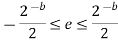
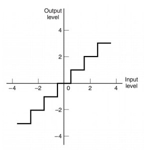
Fig.: Rounding

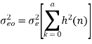
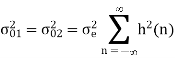
After quantization, we have noise power  as input noise power. Therefore, Output noise power of system is given by
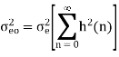
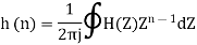
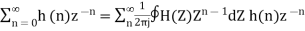
Where h(n) is the impulse response of the system.
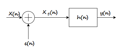
Let error E(n) be output noise power due to quantization Error
E(n)= e(n)*h(n) = 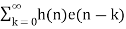
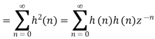
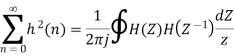
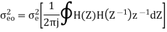
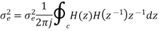
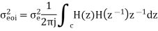
The variance of error E(n) is called output noise power 
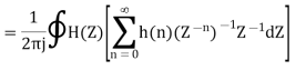
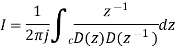
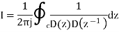
By Parseval’s theorem,
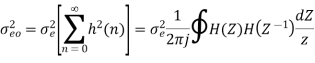
When the closed contour integration is evaluated using the method of residue by taking only the poles that lie inside the unit circle.
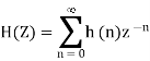
The z-transform of h(n) will be
Examples
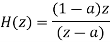
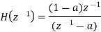
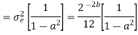
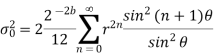
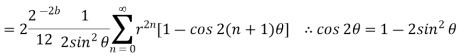
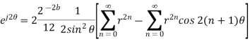
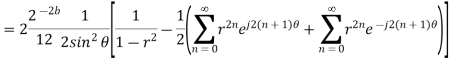
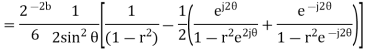
The output signal of an A/D converter is passed through a first order low pass filter, with transfer function given by H(z)= (1-a) z/(z-a) for 0<a<1. Find the steady state output noise power due to quantization at the output of the digital filter.

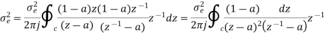
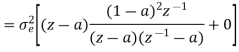
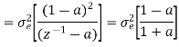
Where:
 = 2-2b/12
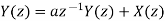
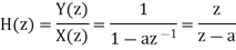
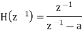
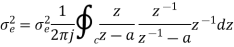
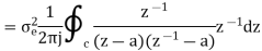
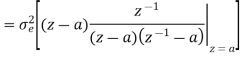
Find the steady state variance of the noise in the output due to quantization of input for the first order filter. y(n)= ay(n-1) + x(n)
The impulse response for the above filter is given by h(n) = anu(n)

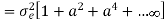
Taking z-transform on both sides we get
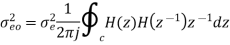
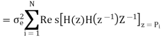
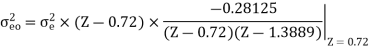
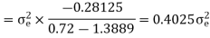
The output of the A/D converter is applied to a digital filter with the system function H(z) = 0.45z/z-0.72. Find the output noise power of the digital filter, when the input signal is quantized to 7 bits.
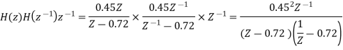
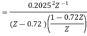
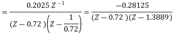
The poles of H(Z)H(Z-1) Z-1 are p1 = 0.72 and p2 = 1.3889
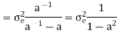
Output noise power due to input quantization
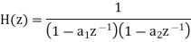
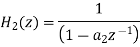
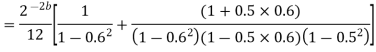
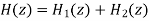
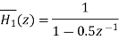
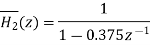
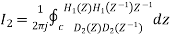
Consider the transfer function H(z) = H1(z)H2(z) where H1(z) = [1/1-a1z-1] and H2(z)=[1/1-a2z-1]. Find the output round off noise power. Assume 1 0.5 and 2 0.6 and find output round off noise power.
The round off noise model for H(z) = H1(z)H2(z) is given by, From the realization we can find that the noise transfer function seen by noise source e1(n) is H(z), where,
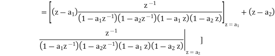
The total steady state noise variance can be obtained we have


If a1 and a2 are less than the poles z=1/a1 and z=1/a2 lies outside of the circle |z|=1. So, the residue of H(z) H(z-1) z-1 at z=1/a1 and z=1/a2 are zero. Consequently, we have

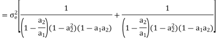
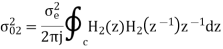
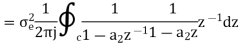
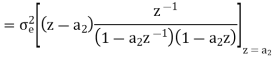

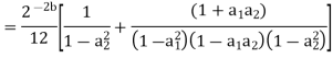
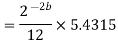
The steady state noise power for a1 0.5, a2 0.6 is given by
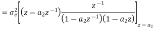
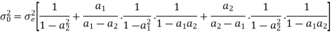
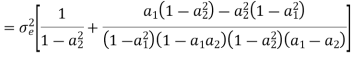
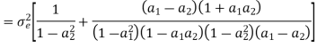
Draw the quantization noise model for a second order system H(z) = 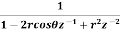 and find the steady state output noise variance.
The quantization noise model is, we know,
Both noise sources see the same transfer function
H(z) = 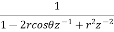
The impulse response of the transfer function is given by
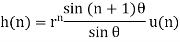
The steady state output noise variance is given by

But we also know that

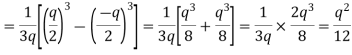
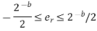
Probability density function for round off error in A/D conversion is
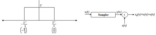
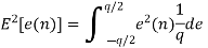
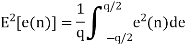
If rounding is used for quantization, which is bounded by -q/2 e(n) q/2, then the error lies between -q/2to q/2 with equal probability, where q is the quantization step size.
Properties of analog to digital conversion error, e(n):
- The error sequence e(n) is a sample sequence of a stationary random process.
- The error sequence is uncorrelated with x(n) and other signals in the system.
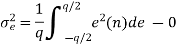
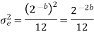
- The error is a white noise process with uniform amplitude probability distribution over the range of quantization error. The variance of e(n) is given by
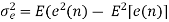
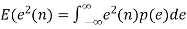
 = Average of e2(n)
 = Mean value of e(n)
For rounding, e(n) lies between -q/2 and q/2 with equal probability
p(e)=1/q


The above equation is known as the steady state noise power due to input quantization
q=R/2b is the two’s compliment representation
q=R/2b-1 is the sign magnitude or one’s compliment representation
R is the range of analog signal to be quantized
We know that the IIR Filter is characterized by the system function
H(z)= 
After quantizing
H(z)q = 
Where [ak]q = ak ak
[bk]q = bk bk
The quantization of filter coefficients alters the positions of the poles and zeros in z-plane.
1. If the poles of desired filter lie close to the unit circle, then the quantized filter poles may lie outside the unit circle leading into instability of filter.
2. Deviation in poles and zeros also lead to deviation in frequency response.
Examples
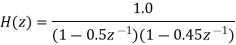
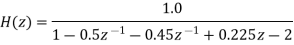
Consider a second order IIR filter with H(z) =  . Find the effect on quantization on pole locations of the given system function in direct form and in cascade form. Take b=3bits.
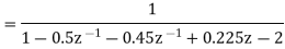
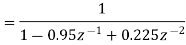
Given that
H(z) = 
H(z) = 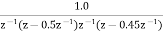
H(z) = 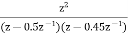
The roots of the denominator of H(z) are the original poles of H(z). Let the original poles of H(z) be p1 and p2. Here p1=0.5 and p2=0.45.
Direct Form I
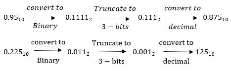
Let us quantize the coefficients by truncation.
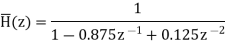
Let  be the transfer function of the IIR system after quantizing the coefficients.
Let 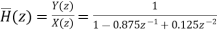
On cross multiplying the above equations we get


Cascade Form

In cascade realization the system can be realized as cascade of first order sections.
Where 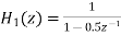 and
and 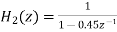


 Let us quantize the coefficients of
  and
and  by truncation

Let  and
and  be the transfer function of the first order sections after quantizing the coefficients
Let 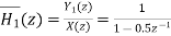
On cross multiplication of above equation, we get
- We know that the limit cycle oscillation is caused by rounding the result of multiplication.
- The limit cycle occurs due to the overflow of adder is known as overflow limit cycle oscillations.
- Several types of limit cycle oscillations are caused by addition, which makes the filter output oscillate between maximum and minimum amplitudes.
Let us consider 2 positive numbers n1 & n2
n1 =0.1117/8
n2 =0.1106/8
n1 + n2 = 1.101-5/8 in sign magnitude form
The sum is wrongly interpreted as a negative number.
The transfer characteristics of a saturation adder is shown in fig below where n is the input to the adder and f(n) is the corresponding output
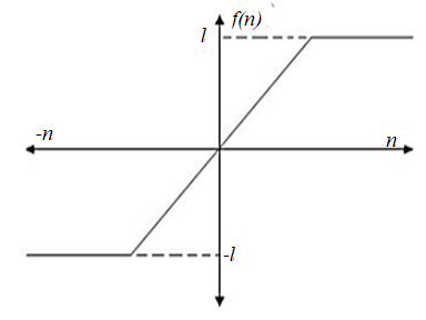
Fig: Saturation adder transfer characteristics
From the transfer characteristics, we find that when overflow occurs, the sum of adder is set equal to the maximum value.
Zero input limit cycle oscillations: The arithmetic operations produces oscillations even when the input is zero or some non zero constant values. Such oscillations are called zero input limit cycle oscillations.
Overflow limit cycle oscillations: The limit cycle occurs due to the overflow of adder is known as overflow limit cycle oscillations.
Dead Band: The limit cycle occurs as a result of quantization effect in multiplication. The amplitude of the output during a limit cycle is confined to a range of values called the dead band of the filter.
Consider a first order filter
y(n)= ay(n-1) + x(n); n>0
After rounding the product
yq(n)= Q[a*y(n-1)] + x(n)
The round
Where, er is the difference between the quantized value and the actual value.
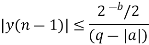
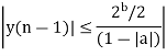
The dead band of the filter for the limit cycle oscillations are
Q[ay(n-1)-ay(n-1)] ≤ 2-b/2
Q[ay(n-1)] = y(n-1), a>0
=-y(n-1), a<0
|y(n-1) | -a|y(n-1) | ≤ 2-b/2
y(n-1) (1-|a|) ≤ 2-b/2
Dead band of the filter
Example
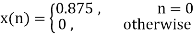
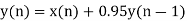
Consider a 1st order FIR system equation y(n) x(n) ay (n 1) with x(n) =0.875 for n=0 and 0 otherwise. Find the limit cycle effect and the dead band. Assume b=4 and a=0.95.
Sol:
Dead band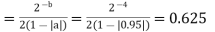
 |  |  |  |  (round off to 4-biits) | 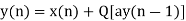 |
0 | 0.875 | 0 | 0 | 0.0000 |  |
1 | 0 | 0.8125 | 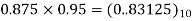 |  |  |
2 | 0 | 0.8125 |  |  |  |
3 | 0 | 0.75 | 0.75×09.5=  |  |  |
4 | 0 | 0.6875 | 0.6875×0.95-  |
 |  |
5 | 0 | 0.625 |  |  |  |
6 | 0 | 0.625 |  |  |  |
The dead band of the filter is 0.625. When n 5 the output remains constant at 0.625 causing limit cycle oscillations.
Saturation arithmetic eliminates limit cycles due to overflow, but it causes undeniable signal distortion due to the non linearity of the clipper. In order to limit the amount of non linear distortion, it is important to scale input signal and unit sample response between input and any internal summing node in the system to avoid overflow
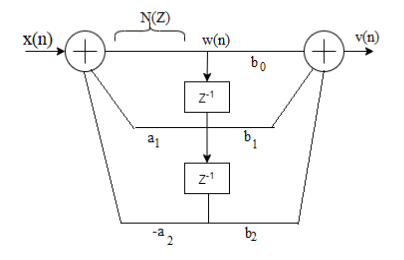
Let us consider a second order IIR filter as shown in the above figure. Here a scale factor S0 is introduced between the input x(n) and the adder 1 to prevent overflow at the output of adder 1.
Now the overall input-output transfer function is
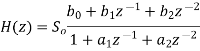

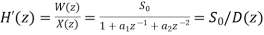
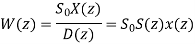
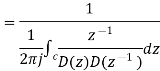
Where: S(z)=1/D(z)
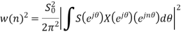
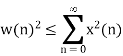
Using Schwartz inequality
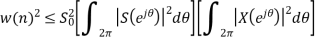
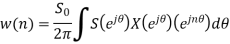
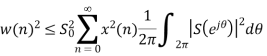
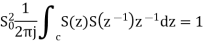
Applying Parseval’s Theorem
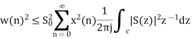
If z=ejΘ then dz=j ejΘ dΘ
Which gives
dΘ=dz/jz
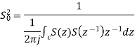
By substituting the values
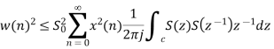
When

Key takeaway
- Because of the process of scaling, the overflow is eliminated. Here so is the scaling factor for the first stage.
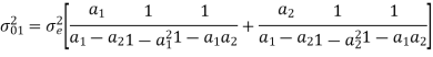
- Scaling factor for the second stage = S01 and it is given by S201=1/S20I2
Examples
For the given transfer function H(z)=  . Find scaling factor so as to avoid overflow in the adder ‘1’ of the filter.
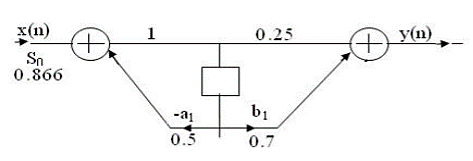
Given D(z)= 1-0.5z-1
D(z‑1)1-0.5z
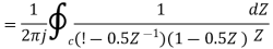
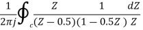
Residue of
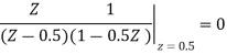
I=1.3333
S0=1/√I
S0=1/√1.3333=0.866
Consider the recursive filter shown in fig. The input x(n) has a range of values of ±100V, represented by 8 bits. Compute the variance of output due to A/D conversion process.
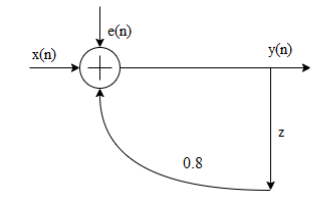
Given the range is ±100V
The difference equation of the system is given by y(n)= 0.8y(n-1)+x(n) whose impulse response h(n) can be obtained by
h(n)= (0.8) n u(n)
Quantization step size= (range of signal)/ (No. Of quantization levels)
= 200/28
=0.78125
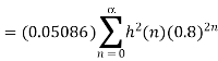
Variance of the error signal
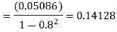
 = 0.05086
Variance of output
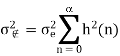
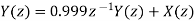
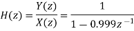
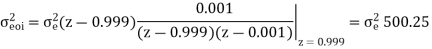
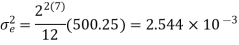
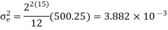
The input to the system y(n)=0.999y(n-1)+x(n) is applied to an ADC. What is the power produced by the quantization noise at the output of the filter if the input is quantized to a) 8 bits b)16 bits.
y(n)=0.999y(n-1)+x(n)
Taking z-transform on both sides
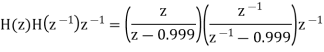
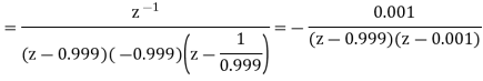
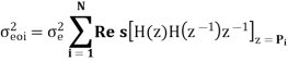
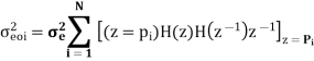
Output noise power due to input quantization 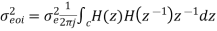
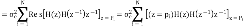
Where p1,p2,……pN are poles of H(z)H(z-1 )z-1 , that lies inside the unit circle in z-plane
a)  bits (Assuming including sign bit)
b) b+1=16 bits
Find the effect of coefficient quantization on pole locations of the given second order IIR system, when it is realized in direct form I and in cascade form. Assume a word length of 4 bits through truncation. H(z)= 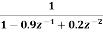
Let b=4 bits including a sign bit
Integer part
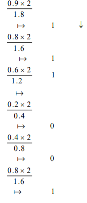
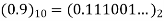
After truncation we get (0.111)2 = (0.875)10
(0.2)10 = (0.00110…)2
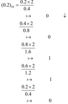
After truncating we get
(0.001)2 = (0.125)10
The system function after coefficient quantization is
H(z)= 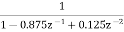
Now the pole locations are given by z1=0.695 and z2=0.178
Cascade form
H(z)= 
(0.5)10= (0.1000)2
After truncation we get
(0.100)2 = (0.5)10
After truncation we get (0.011)2 = (0.375)10
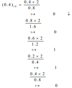
(0.4)10 = (0.01100…)2
The system function after coefficient quantization is
H(z)= 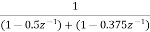
The pole locations are given by z1=0.5 and z2=0.375 on comparing the poles of the cascade system with original poles we can say that one of the poles is same and other pole is very close to original pole.
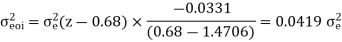
A LTI system is characterized by the difference equation y(n)=0.68y(n-1)+0.5x(n). The input signal x(n) has a range of -5V to +5V, represented by 8-bits. Find the quantization step size, variance of the error signal and variance of the quantization noise at the output.
Range R=-5V to +5V = 5-(-5) =10
Size of binary, B= 8 bits (including sign bit)
Quantization step size,
q=R/28=10/28=0.0390625
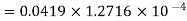
Variance error of the signal = q2/12=1.27116 x 10-4
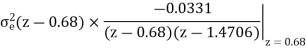
The difference equation governing the LTI system is
Y (n) =0.68y (n-1) +0.15x (n)
On taking z transform of above equation we get


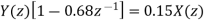
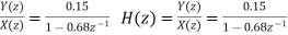
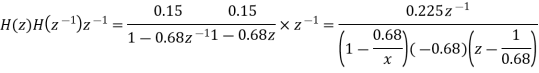
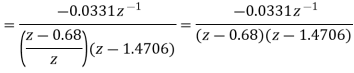
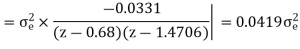
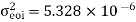
Now, poles of H (z) H (z-1) z-1 are p1=0.68, p2=1.4706 Here, p1=0.68 is the only pole that lies inside the unit circle in z-plane Variance of the input quantization noise at the output.
References:
1. Ifeachor E.C, Jervis B. W, “Digital Signal Processing: Practical approach”, Pearson Publication, 2nd Edition.
2. Li Tan, “Digital Signal Processing: Fundamentals and Applications”, Academic Press, 3rd Edition.
3. Schaum's Outline of “Theory and Problems of Digital Signal Processing”, 2nd Edition.
4. Oppenheim, Schafer, “Discrete-time Signal Processing”, Pearson Education, 1st Edition.
5. K.A. Navas, R. Jayadevan, “Lab Primer through MATLAB”, PHI, Eastern Economy Edition.


