Unit - 4
FIR filter design
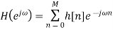
The direct form is obtained from
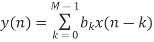
Based on the above equation, we need the current input sample and M−1 previous samples of the input to produce an output point. For M=5, we can simply obtain the following diagram from Equation 1.
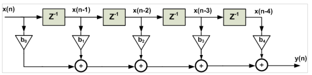
On the other hand, for a linear-phase FIR filter, we observe the following symmetry in coefficients of the difference equation
The structure obtained from the above equation is shown in Figure 2. While Figure 1 requires five multipliers, employing the symmetry of a linear-phase FIR filter, we can implement the filter using only three multipliers. This example shows that for an odd M, the symmetry property reduces the number of multipliers of an (M−1)th-order FIR filter from M to M+1/2.
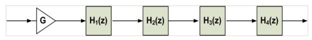
Cascade form
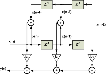
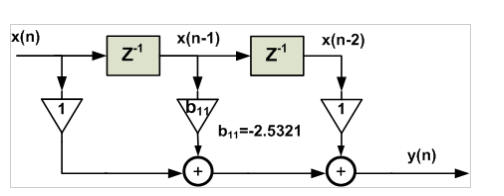
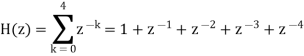
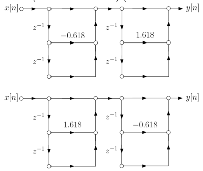
The cascade structure is obtained from the system function H(z). The idea is to decompose the target system function into a cascade of second-order FIR systems. In other words, we need to find second-order systems which satisfy
Where P is the integer part of M/2. For example, M=5, H(z) will be a polynomial of degree four which can be decomposed into two second-order sections. Each of these second-order filters can be realized using a direct form structure. It is desirable to set a pair of complex-conjugate roots for each of the second-order sections so that the coefficients become real.
Assume that we need to implement the nine-tap FIR filter given by the following table using a cascade structure.
k | 4 | 3 and 5 | 2 and 6 | 1 and 7 | 0 and 8 |
 | 0.3333 | 0.2813 | 0.1497 | 0 | -0.0977 |
Solution:
The system function of this filter is

It can be show
Where

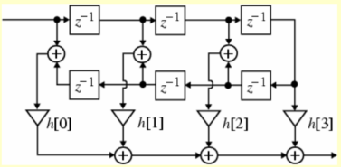
Linear phase structure
The symmetry (or anti symmetry) property of a linear-phase FIR filter can be exploited to reduce the number of multipliers into almost half of that in the direct form implementations • Consider a length-7 Type 1 FIR transfer function with a symmetric impulse response:


We obtain the realization shown below
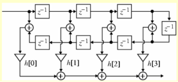
- A similar decomposition can be applied to a Type 2 FIR transfer function
- For example, a length-8 Type 2 FIR transfer function can be expressed as

The Type 1 linear-phase structure for a length-7 FIR filter requires 4 multipliers, whereas a direct form realization requires 7 multipliers
Examples
Q) Draw using the cascade form for the LTI system whose transfer function is
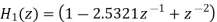
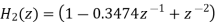
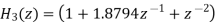
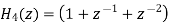
A) Hence H(z) can be factorized as

Although it can be realized with first-order sections, complex coefficients are needed, which implies higher computational cost. To guarantee real-valued coefficients, we group the sections of complex conjugates together.


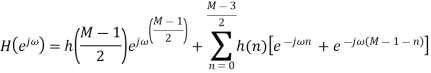
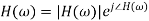
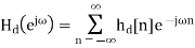
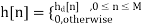
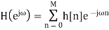
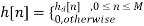
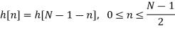
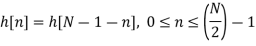
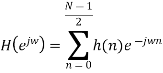
Linear phase is a property of a filter, where the phase response of the filter is a linear function of frequency. The result is that all frequency components of the input signal are shifted in time (usually delayed) by the same constant amount, which is referred to as the phase delay. And consequently, there is no phase distortion due to the time delay of frequencies relative to one another. Linear-phase filters have a symmetric impulse response. The FIR filter has linear phase if its unit sample response satisfies the following condition: h(n) = h(M − 1 − n) n = 0, 1, 2, . . . , N − 1 The Z transform of the unit sample response is given as
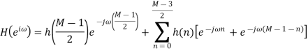
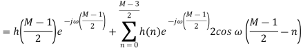
H[z] = 
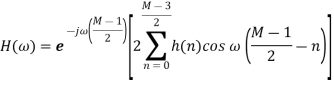
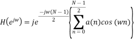
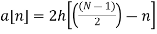
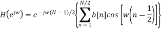
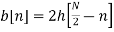
Symmetric impulse response with M=odd Then h(n) = h(M − 1 − n) and (z = ejω)

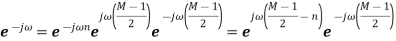

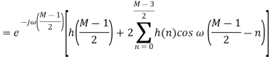
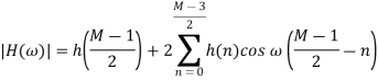
For M=even

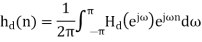
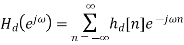
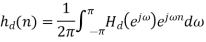
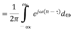
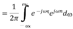
Let the frequency response of the desired LTI ststem we wish to approximate be given by
Where  is the corresponding impulse response.
Consider obtaining a casual FIR filter that approximates  by letting
The FIR filter then has frequency response
Note that sibce we can write
We are actually forming a finite Fourier series approximation to 
Since the ideal  may contain discontinuities at the band edges, truncation of the Fourier series will result in the Gibbs phenomenon.
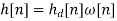
To allow for a less abrupt Fourier series truncation and hence reduce Gibbs phenomenon oscillations, we may generalize h [n] by writing
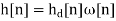
Where  is a finite duration window function of length M +1.
Windowing method
Let the frequency response of the desired LTI ststem we wish to approximate be given by
Where  is the corresponding impulse response.
Consider obtaining a casual FIR filter that approximates  by letting
The FIR filter then has frequency response
Note that sibce we can write
We are actually forming a finite Fourier series approximation to 
Since the ideal  may contain discontinuities at the band edges, truncation of the Fourier series will result in the Gibbs phenomenon.
To allow for a less abrupt Fourier series truncation and hence reduce Gibbs phenomenon oscillations, we may generalize h [n] by writing
Where  is a finite duration window function of length M +1.
Rectangular Window
This is the simplest window function but provides the worst performance from the viewpoint of stopband attenuation. The width of main lobe is 4π/N
ωR(n) = 1 for n=0,1,M-1
= 0 otherwise
Magnitude response of rectangular window is
|WR(ω)| = 
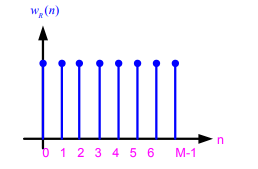
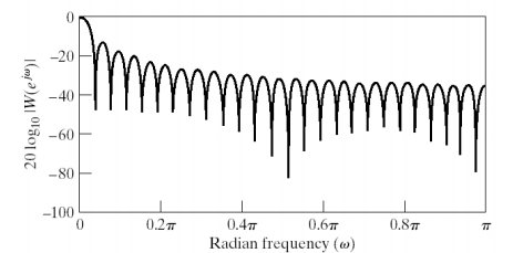
Fig: Rectangular Window
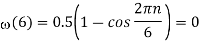
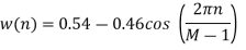
Hanning Window
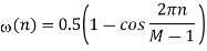
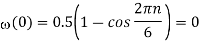
This is a raised cosine window function given by:
W(n) = 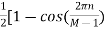 ]
]
W(ω) = 0.5WR(ω) +0.25[WR (ω - ) + WR (ω -
 )]
)]
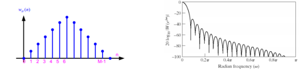
Fig: Hanning Window
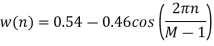
Hamming Window
This is a modified version of the raised cosine window
W(n) = 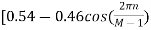 ]
]
W(ω) = 0.54WR(ω) +0.23[WR (ω - ) + WR (ω -
 )]
)]
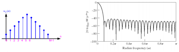
Fig: Hamming Window
Key takeaway
Rectangular | 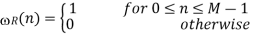 |
Hamming | 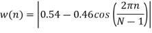 |
Hanning | 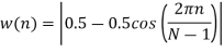 |
Window name | Transition width of main lobe | Min. Stopband attenuation | Peak value of side lobe |
Rectangular |  | -21dB | -21dB |
Hanning |  | -44dB | -31dB |
Hamming |  | -53dB | -41Db |
Barlett |  | -25dB | -25Db |
Blackman |  | -74dB | -57Db |
Example
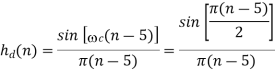
Q1) Design a LPF using rectangular window for the desired frequency response of a low pass filter given by ωc = π/2 rad/sec, and take M=11. Find the values of h(n). Also plot the magnitude response.
Sol:
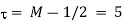
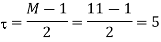
r= M-1/2 = 5
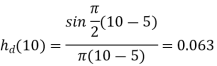
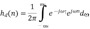
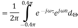
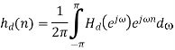
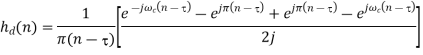
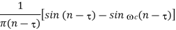
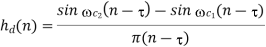
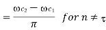
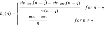
By taking inverse Fourier transform


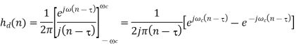

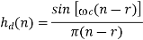
For  and
and 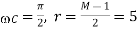
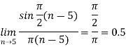
For 
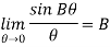
 Using L’Hospital Rule
Where 
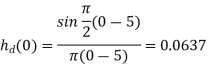
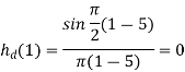
The given window is rectangular window ω(n) = 1 for 0 ≤ n ≤ 10
=0 Otherwise
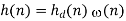
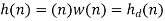
This is rectangular window of length M=11. h(n) = hd (n)ω(n) = hd (n) for 0 ≤ n ≤ 10
H[z]=  =
= 
The impulse response is symmetric with M=odd=11


 |  |  |
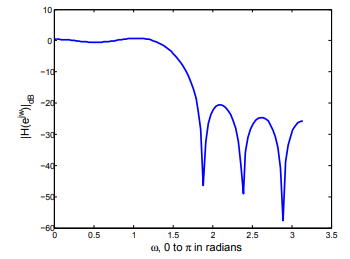
           |            |            |
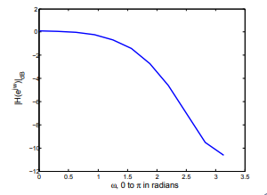
Response
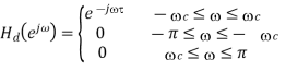
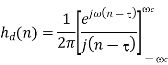
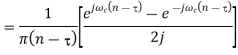
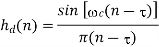
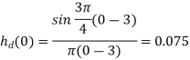
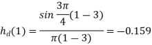
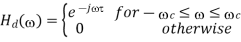
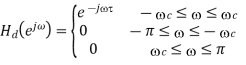
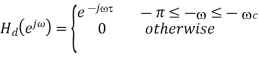
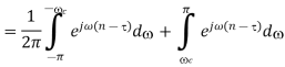
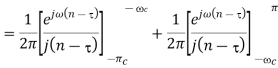
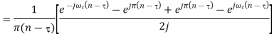
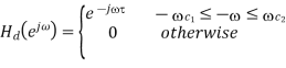
Q2) The desired frequency response of low pass filter is given by Hd (ejω) = e−j3ω − 3π/ 4 ≤ ω ≤ 3π/ 4 and 0 for 3π /4 ≤ |ω| ≤ π Determine the frequency response of the FIR if Hamming window is used with N=7
Sol:
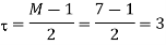
t = M-1/2 = 3


For  and
and 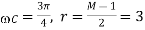
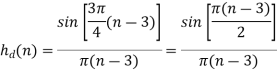
For 
 Using L’Hospital Rule
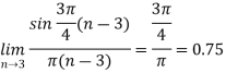
Where 
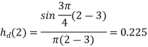
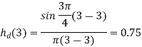
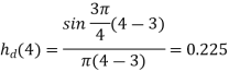


The given window is hamming window
To calculate the value of h(n)


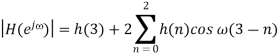
The frequency response is symmetric with M=odd=7


 |  |  |
           |            |        |
RESPONSE
Q3) Design the FIR filter using Hanning window
Sol:

To calculate the value of 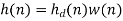


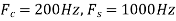
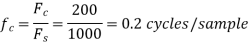
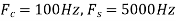
Q4) Design an FIR filter (lowpass) using rectangular window with passband gain of 0 dB, cut-off frequency of 200 Hz, sampling frequency of 1 kHz. Assume the length of the impulse response as 7.
Sol:


When 
When 
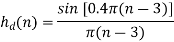
Calculating h(n)
As it is rectangular window h(n) = w(n)=hd(n)=h(n)
For M=7
n |  |
0 | -0.062341 |
1 | 0.093511 |
2 | 0.302609 |
3 | 0.4 |
4 | -0.062341 |
5 | 0.093511 |
6 | 0.302609 |
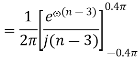
Q5) Using rectangular window design a lowpass filter with passband gain of unity, cut-off frequency of 1000 Hz, sampling frequency of 5 kHz. The length of the impulse response should be 7.
Sol:
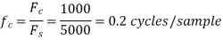


The filter specifications (ωc and M=7) are similar to the previous example. Hence same filter coefficients are obtained.
h (0) =-0.062341, h(1)=0.093511, h(2)=0.302609 h(3)=0.4, h(4)=0.302609, h(5)=0.093511, h(6)=-0.062341
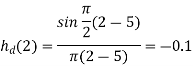
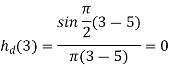
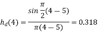
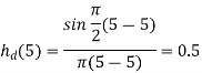
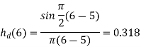
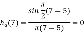
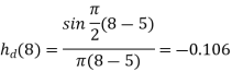
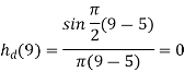
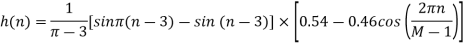
Q6) Design a HPF using Hamming window. Given that cut-off frequency the filter coefficients hd (n) for the desired frequency response of a low pass filter given by ωc = 1rad/sec, and take M=7. Also plot the magnitude response.
Sol:
By taking inverse Fourier transform


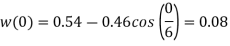
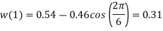
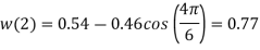
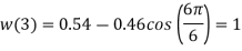
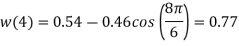
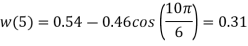
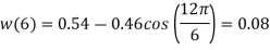
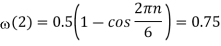
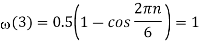
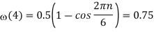
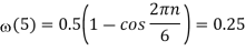
The given window function is Hamming window. In this case
 for
for 
 |  |
0 | -0.00119 |
1 | -0.00448 |
2 | -0.2062 |
3 | 0.6816 |
4 | -0.00119 |
5 | -0.00448 |
6 | -0.2062 |
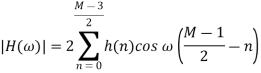
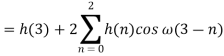
The magnitude response of a symmetric FIR filter with  is
is
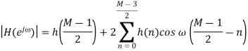
For M=7


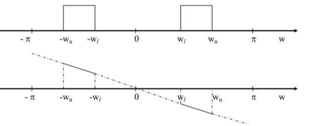
Q7) Design an ideal bandpass filter having frequency response Hde (jω) for π/ 4 ≤ |ω| ≤ 3π/ 4. Use rectangular window with N=11 in your design.
Sol:

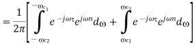
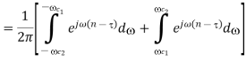
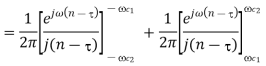
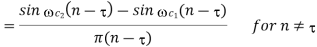
The length of the filter with given is related by
And 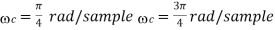
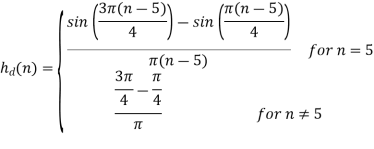
The given window is rectangular hence
For n=0,1,2,…,10 estimate the FIR filter coefficients h(n).
The frequency sampling method is use to design recursive and non-recursive FIR filters for both standard frequency selective filters and with arbitrary frequency response. The main idea of the frequency sampling design method is that a desired frequency response can be approximated by sampling it at N evenly spaced points and then obtaining N-point filter response.
A continuous frequency response is then calculated as an interpolation of the sampled frequency response. The approximation error would then be exactly zero at the sampling frequencies and would be finite in frequencies between them. The smoother the frequency response being approximated, the smaller will be the error of interpolation between the sample points.
There are two distinct types of Non-Recursive Frequency Sampling method of FIR filter design, depending on where the initial frequency sample occurred. The type 1 designs have the initial point at ω=0, whereas the type 2 designs have the initial point at f=1/2N or ω=π/N.
Procedure for Type I design
Choose the desired frequency response

Samples

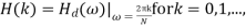
At N points by taking

Where
Generate the sequence H(k). To obtain a good approximation of the desired frequency response, a sufficiently large number of the frequency samples should be taken
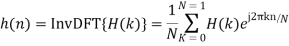
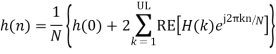
The N points inverse DFT of the sequence H (k) gives the impulse response of the filter h (n). For a practical realization of the filter, samples of impulse response should be real. This can happen if all the complex terms appears in conjugate pairs.
Desired filter coefficients
For linear phase filter with positive symmetrical impulse response,
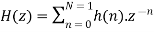
4) take z transform of the impulse response h (n) to get the filter transfer function H (z)
Procedure for Type 2 Design
(Same steps as above expect step 2)
2) Samples  at N points by taking
 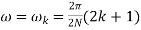 where
where  generate the sequence H (z)

Type 2 frequency samples gives additional flexibility in the design method to satisfy the desired frequency response at a second possible set of frequencies.
Consider a signal that consists of several frequency components passing through a filter.
The phase delay (Tp) of the filter is the amount of time delay each frequency component of the signal suffers in going through the filter.
The group delay (Tg) is the average time delay the composite signal suffers at each frequency.
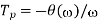
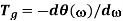
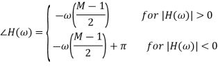
Where Θ(w) is the phase angle
A filter is said to have a linear phase response if,

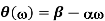
Where α and  are constants
For Example
For ideal LPF
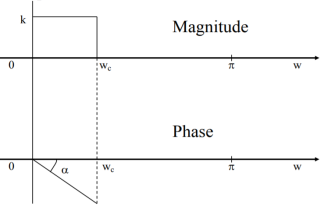
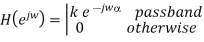
Magnitude response= 
Phase response 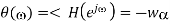
Follows:  Linear phase implies that the output is a replica of x[n] {LPF} with a time shift of .
- Symmetric impulse response will yield near phase FIR filters.
Positive symmetry of impulse response
 n=0,1,…,(N-1)/2 (N odd)
N=0,1,…(N/2)-1 (N even)
Negative symmetry of impulse response:
 n=0,1,…,(N-1)/2 (N odd)
n=0,1,…(N/2)-1 (N even)


Types of FIR linear phase systems
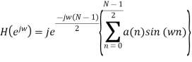
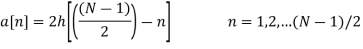
1. Type I FIR linear phase system
The impulse response is positive symmetric and N an odd integer.
The frequency response is

Where 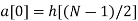
 n=1,2,…,(N-1)/2
2. Type II FIR linear phase system
The impulse response is positive symmetric and N is an even integer
The frequency response is
Where

3. Type III FIR linear phase system
The impulse response is negaitve-symmetric and N an odd integer


Where
Key takeaway
There are two distinct types of Non-Recursive Frequency Sampling method of FIR filter design, depending on where the initial frequency sample occurred. The type 1 designs have the initial point at ω=0, whereas the type 2 designs have the initial point at f=1/2N or ω=π/N.
References:
1. Ifeachor E.C, Jervis B. W, “Digital Signal Processing: Practical approach”, Pearson Publication, 2nd Edition.
2. Li Tan, “Digital Signal Processing: Fundamentals and Applications”, Academic Press, 3rd Edition.
3. Schaum's Outline of “Theory and Problems of Digital Signal Processing”, 2nd Edition.
4. Oppenheim, Schafer, “Discrete-time Signal Processing”, Pearson Education, 1st Edition.
5. K.A. Navas, R. Jayadevan, “Lab Primer through MATLAB”, PHI, Eastern Economy Edition.


