Unit - 3
Different type of line coding and Equalization
When binary data is sent through a link, it is represented by a physical quantity in the transport medium. In electrical links, that's usually a voltage or current; optical systems use the intensity of light; and wireless radio links often use the phase and frequency of a signal carrier. Line coding determines how the binary data is represented on the link.
Numerous coding schemes are available, and which one is best for any given application depends on many factors. Coding can influence the frequency spectrum, the direct current content, and the transition density of the resulting data stream. Coding efficiency determines the required link bandwidth, and the cost of implementation depends on the complexity of the code.
Properties of Binary Data
Mark Density
The mark density (MD) of a binary data pattern is defined as the number of one bits in the pattern, divided by the length of the pattern:
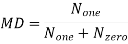
Where NOne is the number of ones in the pattern, and NZero is the number of zeros. The mark density ranges from 0.0 to 1.0, where the extremes are marked by all-zeros (NOne equals 0) and all-ones data (NZero equals 0). Random data is exactly at the middle of the range: It contains as many one bit as zero bits, and its long-term mark density is therefore 0.5. If we look only at a subsection of the random data pattern, however, its mark density can be very different.
Key Takeaways:
- Line coding determines how the binary data is represented on the link.
- The mark density (MD) of a binary data pattern is defined as the number of one bit in the pattern, divided by the length of the pattern:
Unipolar Return to Zero RZRZ
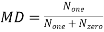
In this type of unipolar signaling, a High in data, though represented by a Mark pulse, its duration T0 is less than the symbol bit duration. Half of the bit duration remains high but it immediately returns to zero and shows the absence of pulse during the remaining half of the bit duration.
It is clearly understood with the help of the following figure.
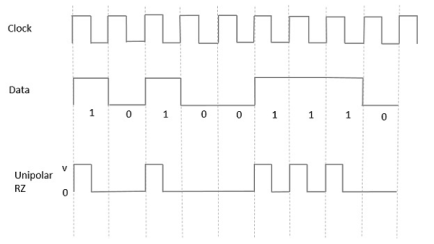
Fig 1: Unipolar RZ
Advantages
The advantages of Unipolar RZ are −
- It is simple.
- The spectral line present at the symbol rate can be used as a clock.
Disadvantages
The disadvantages of Unipolar RZ are −
- No error correction.
- Occupies twice the bandwidth as unipolar NRZ.
- The signal droop is caused at the places where signal is non-zero at 0 Hz
Polar NRZ
In this type of Polar signaling, a High in data is represented by a positive pulse, while a Low in data is represented by a negative pulse. The following figure depicts this well.
Fig 2 Polar NRZ
Advantages
The advantages of Polar NRZ are −
- It is simple.
- No low-frequency components are present.
Disadvantages
The disadvantages of Polar NRZ are −
- No error correction.
- No clock is present.
- The signal droop is caused at the places where the signal is non-zero at 0 Hz.
Polar RZ
In this type of Polar signaling, a High in data, though represented by a Mark pulse, its duration T0 is less than the symbol bit duration. Half of the bit duration remains high but it immediately returns to zero and shows the absence of pulse during the remaining half of the bit duration.
However, for a Low input, a negative pulse represents the data, and the zero level remains same for the other half of the bit duration. The following figure depicts this clearly.
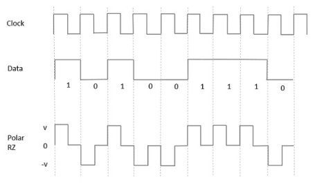
Fig 3 Polar RZ
Advantages
The advantages of Polar RZ are −
- It is simple.
- No low-frequency components are present.
Disadvantages
The disadvantages of Polar RZ are −
- No error correction.
- No clock is present.
- Occupies twice the bandwidth of Polar NRZ.
- The signal droop is caused at places where the signal is non-zero at 0 Hz.
Manchester coding consists of combining the NRZ-L and RZ schemes. Every symbol has a level transition in the middle: from high to low or low to high. Uses only two voltage levels.
Differential Manchester coding consists of combining the NRZ-I and RZ schemes. Every symbol has a level transition in the middle. But the level at the beginning of the symbol is determined by the symbol value. One symbol causes a level change the other does not.

Fig 4 Polar biphase: Manchester and differential Manchester schemes
Key takeaway
- In Manchester and differential Manchester encoding, the transition at the middle of the bit is used for synchronization.
- The minimum bandwidth of Manchester and differential Manchester is 2 times that of NRZ. The is no DC component and no baseline wandering. None of these codes has error detection.
A '1' bit is indicated by making the first half of the signal, equal to the last half of the previous bit's signal i.e. no transition at the start of the bit-time. A '0' bit is indicated by making the first half of the signal opposite to the last half of the previous bit's signal i.e. a zero bit is indicated by a transition at the beginning of the bit-time. In the middle of the bit-time there is always a transition, whether from high to low, or low to high. Each bit transmitted means a voltage change always occurs in the middle of the bit-time to ensure clock synchronisation. Token Ring uses DME and this is why a preamble is not required in Token Ring, compared to Ethernet which uses Manchester encoding.

Bit and Frame Synchronization techniques are used in order to ensure that signals transmitted from one participant of the communication can be correctly decoded by the receiver.
Bit Synchronization
For synchronous transmission, data is not transferred byte-wise so there is no start or stop bits indicating the beginning or end of a character. Instead, there is a continuous stream of bits which have to be split up into bytes. Therefore, the receiver has to sample the received data in the right instant and the sender's and receiver's clocks have to be kept in a synchronized state. As the main task lies in synchronizing sender's and receiver's clocks, bit synchronization is also called clock synchronization.
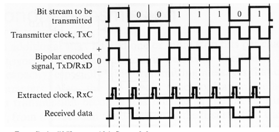
Clock encoding
The most self-evident way to accomplish clock synchronization is to send the clock signal to the receiver. This can be done by adding the signal of the local clock to the encoded signal of the bit stream resulting in a bipolar encoded signal which the receiver will have to interpret. By using this bipolar encoding, it is not necessary to create an additional transmission line just for the clock signal. Each bit span of the bipolar2 signal is dived in the middle by the signal shift of the clock. There are two possible values for each bit span: high-zero and low-zero, denoting logical one and logical zero. The received signal will contain enough information for the encoder as it can determine the length of a bit by the guaranteed signal change at the end of each bit and it can determine the literal value by distinguishing between a positive or negative signal in the first half of the bit time
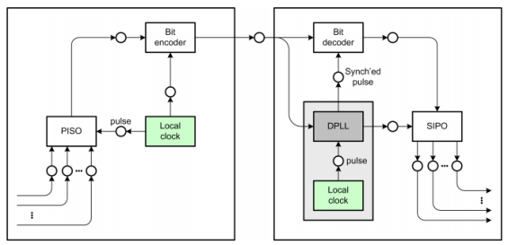
Digital Phase-Locked Loop
The main idea of a digital phase locked loop is that the receiver's clock is reasonably accurate, but should be resynchronized with the sender's clock whenever possible. Unlike the direct clock encoding, there is no direct transmission of the clock signal, but it is possible to extract clock information from the received data signal. It is important that there are enough bit transitions in the received data stream which indicate bit boundaries and make it possible to deduct the duration of a bit time as well as enabling the clock controller to reset the clock to a less diverged signal. This can be ensured by using a bit scrambler which removes long sequences of zeros or one's, but a more convenient way is to use an encoding scheme which ensures a sufficient number of bit transitions like the Manchester encoding
Frame synchronization
In modern computer networks data is not transferred as a simple stream of bits or bytes but in terms of frames or packets. This enables amongst other things packet based routing, error correction and the sharing of one physical medium between multiple clients. As the medium usually is a serial link and does not have a concept of frames or separated data units the sender and receiver have to recognize frame borders in the data stream on the medium. This process is called Frame Synchronization.
Time gap synchronization
The most obvious method for synchronization is leaving a time gap between frames. This is of course only possible if an idle state of the transfer medium is recognizable and distinguishable from for example a long row of zeros. If the bits are encoded using return to zero signalling time gaps cannot be used. While this is simple and easy to implement it has disadvantages too. To make sure each of the communication partners recognizes the time gap as such it has to be long enough compared to the length of one information cell in asynchronous data transfers. This brings a performance penalty. Time gap synchronization is usually used in combination with another method of frame synchronization like packet length indication because it might fail if line noise is encountered and by that needs a backup technique.
Start & End Flags
Frame Synchronization via start and end flags is very widely used. The general idea is to separate the single frames by special data sequences, the flags. These flags are commonly referred to as "STX" which stands for "start-of-text" and "ETX" for "end-of text". Whenever the receiver encounters a STX flag it knows it has detected the beginning of a new frame whilst ETX signals the end of the current frame. In many cases there is no need to distinguish between the start and the end of a frame. If the receiver is currently receiving a frame only an ETX character can be valid and if it is not receiving a frame only the STX character can be valid. Because of that to avoid any overhead STX and ETX are usually chosen to be the same character. Please see Figure 19, “Frame Synchronization via start & end flags” for a graphical representation of a frame embedded in STX and ETX flags.

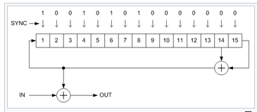
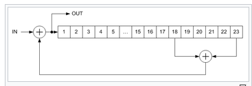
Scrambler
Scrambler is a device that transposes or inverts signals or otherwise encodes a message at the sender's side to make the message unintelligible at a receiver not equipped with an appropriately set descrambling device.
Whereas encryption usually refers to operations carried out in the digital domain, scrambling usually refers to operations carried out in the analog domain. Scrambling is accomplished by the addition of components to the original signal or the changing of some important component of the original signal in order to make extraction of the original signal difficult. Examples of the latter might include removing or changing vertical or horizontal sync pulses in television signals; televisions will not be able to display a picture from such a signal. Some modern scramblers are actually encryption devices, the name remaining due to the similarities in use, as opposed to internal operation.
Types:
- Additive (synchronous) scramblers
Additive scramblers (they are also referred to as synchronous) transform the input data stream by applying a pseudo-random binary sequence (PRBS) (by modulo-two addition). Sometimes a pre-calculated PRBS stored in the read-only memory is used, but more often it is generated by a linear-feedback shift register (LFSR).
- Multiplicative (self-synchronizing) scramblers
Multiplicative scramblers (also known as feed-through) are called so because they perform a multiplication of the input signal by the scrambler's transfer function in Z-space. They are discrete linear time-invariant systems. A multiplicative scrambler is recursive, and a multiplicative descrambler is non-recursive. Unlike additive scramblers, multiplicative scramblers do not need the frame synchronization, that is why they are also called self-synchronizing.
This is a form of distortion of a signal, in which one or more symbols interfere with subsequent signals, causing noise or delivering a poor output.
Causes of ISI
The main causes of ISI are −
- Multi-path Propagation
- Non-linear frequency in channels
The ISI is unwanted and should be completely eliminated to get a clean output. The causes of ISI should also be resolved in order to lessen its effect.
To view ISI in a mathematical form present in the receiver output, we can consider the receiver output.
The receiving filter output y(t)y(t) is sampled at time ti=iTb (with i taking on integer values), yielding –
y(ti)= μ∑akp(iTb−kTb)
= μai+μ∑akp(iTb−kTb)
In the above equation, the first term μai is produced by the ith transmitted bit.
The second term represents the residual effect of all other transmitted bits on the decoding of the ith bit. This residual effect is called as Inter Symbol Interference.
In the absence of ISI, the output will be −
y(ti)=μai
This equation shows that the ith bit transmitted is correctly reproduced. However, the presence of ISI introduces bit errors and distortions in the output.
While designing the transmitter or a receiver, it is important that you minimize the effects of ISI, so as to receive the output with the least possible error rate.
Equalization
For reliable communication, we need to have a quality output. The transmission losses of the channel and other factors affecting the quality of the signal. The most occurring loss, as we have discussed, is the ISI.
To make the signal free from ISI, and to ensure a maximum signal to noise ratio, we need to implement a method called Equalization.
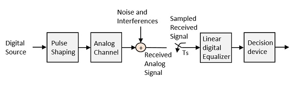
Fig 5: Equalization
The noise and interferences which are denoted in the figure, are likely to occur, during transmission. The regenerative repeater has an equalizer circuit, which compensates the transmission losses by shaping the circuit. The Equalizer is feasible to get implemented.
Key takeaway
The main causes of ISI are −
- Multi-path Propagation
- Non-linear frequency in channels
To make the signal free from ISI, and to ensure a maximum signal to noise ratio, we need to implement a method called Equalization.
An eye diagram or eye pattern is simply a graphical display of a serial data signal with respect to time that shows a pattern that resembles an eye.
The signal at the receiving end of the serial link is connected to an oscilloscope and the sweep rate is set so that one- or two-bit time periods (unit intervals or UI) are displayed. This causes bit periods to overlap and the eye pattern to form around the upper and lower signal levels and the rise and fall times. The eye pattern readily shows the rise and fall time lengthening and rounding as well as the horizontal jitter variation.

Fig 6: Eye diagram
Nyquist proposed a condition for pulses p(t) to have zero–ISI when transmitted through a channel with sufficient bandwidth to allow the spectrum of all the transmitted signal to pass. Nyquist proposed that a zero–ISI pulse p(t) must satisfy the condition
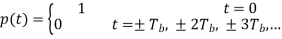
A pulse that satisfies the above condition at multiples of the bit period Tb will result in zero– ISI if the whole spectrum of that signal is received. The reason for which these zero–ISI pulses (also called Nyquist–criterion pulses) cause no ISI is that each of these pulses at the sampling periods is either equal to 1 at the centre of pulse and zero the points other pulses are centred.
There is a set of pulses known as raised–cosine pulses that satisfy the Nyquist criterion and require slightly larger bandwidth than what a sinc pulse requires.
The spectrum of these pulses is given by
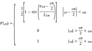
Where ω b is the frequency of bits in rad/s (ω b = 2 /Tb), and x is called the excess bandwidth and it defines how much bandwidth would be required above the minimum bandwidth that is required when using a sinc pulse. The excess bandwidth ω x for this type of pulses is restricted between


For ωx = 0 the wave is rect function and the pulse is sinc function. When ωx = ωb/2 the spectrum is sinc function but decays early. The expense for having a pulse that is short in time is that it requires a larger bandwidth than the sinc function. The waveform is shown below


Fig 7 Pulse and its spectrum for ωx = ωb/2 and ωx = 0
The roll-off factor is the ratio of extra bandwidth required for the pulses to the minimum bandwidth required by sinc function.

Key takeaway
The roll-off factor is the ratio of extra bandwidth required for the pulses to the minimum bandwidth required by sinc function.
Equalization is a technique used to combat inter symbol interference (ISI). An Equalizer within a receiver compensates for the average range of expected channel amplitude and delay characteristics. Equalizers must be adaptive as the channel is generally unknown and time varying. ISI has been recognized as the major obstacle to high-speed data transmission over mobile radio channels.
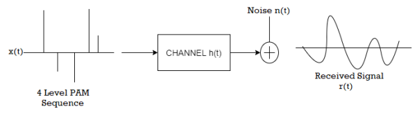
The goal of equalizers is to eliminate inter-symbol interference (ISI) and the additive noise as much as possible.
- Inter-symbol interference arises because of the spreading of a transmitted pulse due to the dispersive nature of the channel, which results in overlap of adjacent pulses.
- In Figure, there is a four‐level pulse amplitude modulated signal (PAM), x(t). This signal is transmitted through the channel with impulse response h(t). Then noise n(t) is added. The received signal r(t) is a distorted signal.
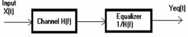
Equalizers are used to overcome the negative effects of the channel. In general, equalization is partitioned into two broad categories;
1. Maximum likelihood sequence estimation (MLSE) which entails making measurement of channel impulse response and then providing a means for adjusting the receiver to the transmission environment. (Example: Viterbi equalization)
2. Equalization with filters, uses filters to compensate the distorted pulses. The general channel and equalizer pair is shown in Figure.
The purpose of the equalizer filter is to shape the frequency characteristics of the voice signals transmitted through the IP phone system. Transducers in telephone audio devices apply an undesirable frequency response to the voice signals, and the equalizer filter is designed to compensate for this response. In this section, we discuss the filter specifications and design process. The user of the IP phone software specifies the frequency magnitude response of the equalizer filter. The user needs to measure the transducer frequency response of the telephone device. Based on the measured frequency response, the user needs to determine what frequency response the equalizer filter should have to ensure that the overall frequency response of the voice signals meets the user requirements.
We initially designed the equalizer filter to meet the specific frequency magnitude response provided by the IP phone user for whom the development was being done. However, we also ensured that both the design process and the filter implementation were generic enough so that the equalizer filter could be used again to meet different frequency requirements with minimal additional effort. When processing real-time voice signals, we would like to minimize the filter delay and phase distortion. A minimum phase filter minimizes the filter group delay and a linear phase filter prevents phase distortion.
Our initial filter specifications did not require a linear phase response. Hence, we designed a minimum phase filter in order to minimize the overall filter delay. In addition, minimum phase filters do not have the coefficient symmetry constraints that linear phase filters do, allowing for greater design flexibility. The filter design process was influenced by several software constraints. The primary software constraints included the memory requirements and processor consumption of the equalizer filter. These considerations are especially important in large software systems where resources can be limited and should be used with maximum efficiency.
For example, a higher order filter will achieve a closer approximation to the desired frequency magnitude response, but will require more memory space to store the coefficients and more processor cycles to compute a single output sample, than a lower order filter. There is a tradeoff between achieving a frequency response closely matching the original filter specifications and using minimal processor and memory resources.
Given the filter specifications, we chose to implement the equalizer filter as a minimum phase FIR filter. Although FIR filters are more computationally intensive than IIR filters, they are guaranteed to be stable and are particularly simple to implement on a DSP. We designed the equalizer filter to be a minimum phase filter. This implies that the filter magnitude response and phase response uniquely specify each other to within a scale factor. Minimum phase systems are causal and stable and must have all their poles and zeros within the unit circle on the complex plane. We used the window method to calculate the FIR coefficients. This method employs the Fourier transform relationship between the impulse response hd(n), and the frequency response of the filter Hd(w).
Hd(n) = 1/2π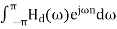
Given the desired filter frequency response, the Fourier transform can be used to compute the time domain impulse response hd(n). However, this response is an ideal response and includes more coefficients than we can retain for the filter implementation. Therefore, we truncate the impulse response to the desired filter order by multiplying it with a window function. An example of such a window function is the rectangular window, which retains all samples within the width of the window and discards all other samples. Multiplication of two signals in the time domain corresponds to convolution of the signals in the frequency domain. The multiplication of the filter impulse response with a window function distorts the filter frequency response because of this convolution. Equation below represents this relationship between the ideal filter response Hd(w), the window function W(w), and the actual filter response H(w):
h(n)=hd(n) w(n)
H(ω)= H (ω) *W (ω)
The frequency distortion resulting from windowing depends on the window function. For example, the more coefficients we retain, or equivalently, the higher the filter order, the closer the filter frequency response is to the ideal response. Therefore, ideally the width of the window function w(n) is as large as possible so that most of the samples of the impulse response are retained, and H(n) approaches Hd(n). However, the filter order should be kept small in order to minimize the number of computations required to produce each filtered output sample. Retaining more coefficients also requires more memory for their storage. In selecting the filter order, we need to consider the practical implementation constraints in addition to our desire to approximate the ideal frequency response as closely as possible. For the equalizer filter we implemented, the filter order is a programmable parameter to allow for flexibility when designing the equalizer filter according to the user specific requirements.
Adaptive equalizers assume channel is time varying channel and try to design equalizer filter whose filter coefficients are varying in time according to the change of channel, and try to eliminate ISI and additive noise at each time. The implicit assumption of adaptive equalizers is that the channel is varying slowly.

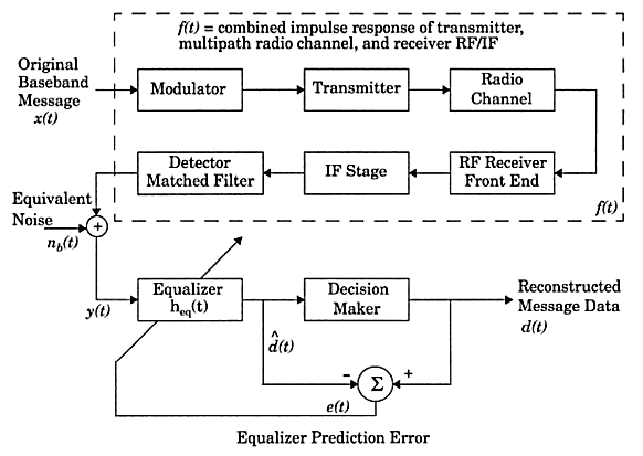
Fig 8 Block Diagram of Adaptive Equalizer
As the mobile fading channels are random and time varying, equalizers must track the time varying characteristics of the mobile channel, and thus are called adaptive equalizers.
Working principles of adaptive equalizers
The working principles of adaptive equalizers are in the following:
- The received signal is applied to receive filter. In here, receive filter is not matched filter. Because we do not know the channel impulse response. The receive filter in here is just a low‐pass filter that rejects all out of band noise.
- The output of the receiver filter is sampled at the symbol rate or twice the symbol rate.
- Sampled signal is applied to adaptive transversal filter equalizer. Transversal filters are actually FIR discrete time filters.
- The object is to adapt the coefficients to minimize the noise and intersymbol interference (depending on the type of equalizer) at the output.
- The adaptation of the equalizer is driven by an error signal.
Operation mode of adaptive equalizers
There are two modes that adaptive equalizers work
1. Decision Directed Mode: This means that the receiver decisions are used to generate the error signal.
2. Decision directed equalizer adjustment is effective in tracking slow variations in the channel response.
However, this approach is not effective during initial acquisition.
- Training Mode: To make equalizer suitable in the initial acquisition duration, a training signal is needed. In this mode of operation, the transmitter generates a data symbol sequence known to the receiver. The receiver therefore, substitutes this known training signal in place of the slicer output. Once an agreed time has elapsed, the slicer output is substituted and the actual data transmission begins. Initially, a known, fixed length training sequence is sent by the transmitter so that the receiver’s equalizer may average to a proper setting. The training sequence is a pseudo random signal or a fixed, prescribed bit pattern. Immediately following the training sequence, the user data is sent.
- Tracking mode: When the data of the users are received, the adaptive algorithm of the equalizer tracks the changing channel. As a result of this, the adaptive equalizer continuously changes the filter characteristics over time. Equalizers are widely used in TDMA Systems.
Algorithm for Adaptive Equalization
Performance measures for an algorithm
- Rate of convergence
- Mis adjustment
- Computational complexity
- Numerical properties
Factors dominate the choice of an equalization structure and its algorithm
- The cost of computing platform
- The power budget
- The radio propagation characteristics
The speed of the mobile unit determines the channel fading rate and the Doppler spread, which is related to the coherent time of the channel directly. The choice of algorithm, and its corresponding rate of convergence, depends on the channel data rate and coherent time. The number of taps used in the equalizer design depends on the maximum expected time delay spread of the channel. The circuit complexity and processing time increases with the number of taps and delay elements. Three classic equalizer algorithms: zero forcing (ZF), least mean squares (LMS), and recursive least squares (RLS) algorithms.
Decision-Directed (DD) equalization is the most primitive Blind Equalization (BE) method for the cancel ling of Inter-Symbol-Interference (ISI) in data communication systems. Even though DD equalizers are believed to be unable to open the channel eye when it is initially closed, this does not seem to be true in the case of Constant-Modulus (CM) constellations (pure phase modulation). We investigate the shape of the DD cost function in this case and obtain several interesting results that indicate that the DD algorithm should be capable of opening a closed channel eye in the CM case. Based on this fact, we propose a novel hybrid CMA-DD equalization scheme that offers an appealing alternative to the Generalized Sato (GSATO) algorithm for QAM constellations. Our theoretical claims about the performance of DD equalizers as well as the performance of our novel scheme are verified through computer simulations.
Consider the baseband representation of a QAM digital communication system, as depicted in figure. The channel is assumed to be a linear filter whose z transform of its impulse response is C(z-1) and the equalizer is also a FIR filter with corresponding z transform W(z-1). We denote by {ai}; {xi} and {yi} the transmitted (input), received and equalized sequence of data, respectively. If the channel equalizer is assumed to have N taps, the equalizer output can be written as yk = XHk Wk, where XHk = [xk, xk-1…. xk-N+1] and Wk is a NX1 vector containing the equalizer taps at time instant k. We also denote by s the overall channel-equalizer impulse response: si = ci*wi (denotes convolution). In terms of s, the equalizer output can be written as
yk=s*ak = 
In BE, the input sequence {ai} is identified based only on the received sequence {xi} and some a prior knowledge of the statistics of {ai}. A strong identifiability result is seen, where it was stated that a necessary and sufficient condition for zero-forcing equalization in the noiseless case is that the following two condition
E(|y|2) = E(|a|2)
|K(y)|=|K(a)|
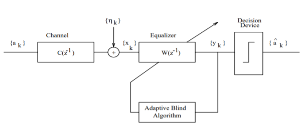
Fig:9 A typical blind equalization
Where E(.) denotes statistical expectation and K(.) is the Kurtosis of a process (K (zi) = E (|zi|4-2E2 (|zi|2)- E(z2i) 2). It turns out that in the case of a sub-Gaussian (K(a) < 0) and symmetrical (E(a2) = 0) input distribution, a noiseless channel and an infinite-length equalizer, the Godard cost function defined as
J(p)(W) = 1/2p [E (|yk|p- rp)2]
In the particular case p = 2 is a convex function of s whose global minima are optimal settings (s = e j )
)
A decision feedback equalizer (DFE) is a nonlinear equalizer that uses previous detector decisions to eliminate the ISI on pulses that are currently being demodulated. • The basic idea of a DFE is that if the values of the symbols previously detected are known (past decisions are assumed to be correct), then the ISI contributed by these symbols can be cancelled out exactly the output of the forward filter by subtracting past symbols values with appropriate weighting. In
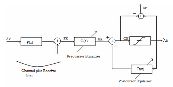
Fig 10 Block diagram of Adaptive DFE
If we look at Figure above, we see that the estimated signal sequence becomes
Qk = 
{ci}s are coefficients of the precursor equalizer, {di} are coefficients of the postcursor equalizer. N is the number of precursor equalizer coefficients and M is the number of postcursor equalizer coefficients. Adaptive DFE algorithm is similar to stochastic gradient algorithm, with the important difference that the input to the causal portion of the filter is the decisions rather than the output of the precursor equalizer filter. This difference will obviously change the desired tap coefficients as well as reduce the noise enhancement due to equalization.
Partial-response signaling (PRS), also known as correlative level-coding, is a signaling scheme first proposed for data communications. In contrast to a conventional pulse-amplitude modulation system, in which no inter-symbol interference (ISI) is allowed, a PRS system introduces a controlled amount of [SI to the signal. This ISI is known and cm be removed at the receiver. By relaxing the condition of zero ISI, certain beneficial effects can be attained through convenient spectrally shaping. Two examples of these effects are providing more similarity between the spectrum of the transmitted signal and the frequency response of the channel and realizing minimum-bandwidth transmission systems in practice.
The operation of a PRS system can be understood by the model shown in figure. In this model, an FR filter is employed to introduce the ISI, whereas a low-pass filter band-limits the resulting signal. To have the ISI exclusively controlled by the FIR filter, the low-pass filter, H (a), should be designed such that it preserves the relative sample values.
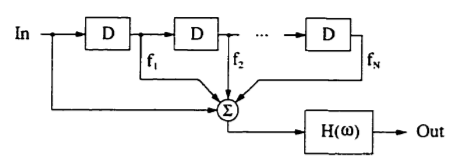
Fig 11 A partial-response encoder model
The operator D reflects a time-step delay of T = l/fs, where f, is the sampling frequency. Using this notation, the resulting transfer function of the FIR filter becomes a polynomial of D
F(D) = 1+  1=Fl (D)
Where fN  0 is assumed. We shall refer to the above polynomial as the "coding polynomial" of the PRS system.
It is clear that a PRS system results in an increase in the number of output levels. In addition to a drop in the power of the signal, the implementation complexity will increase as the number of these levels increases. As a result, this number should be kept to a minimum. Without any loss of generality, we shall normalize the peak values of the multi-level partial-response (PR) signal to  by considering a low-frequency gain equal to
h= 
Case Study
QAM for Wireless Communication
Another major development occurred in 1987 when Sundberg, Wong and Steele published a pair of papers. Considering QAM for voice transmission over Rayleigh fading channels, the first major paper considering QAM for mobile radio applications. In these papers, it was recognized that when a Gray code mapping scheme was used, some of the bits constituting a symbol had different error rates from other bits. Gray coding is a method of assigning bits to be transmitted to constellation points in an optimum manner. For the 16-level constellation two classes of bits occurred, for the 64-level three classes and so on. Efficient mapping schemes for pulse code modulated (PCM) speech coding was, discussed where the most significant bits (MSBs) were mapped onto the class with the highest integrity. A number of other schemes including variable threshold systems and weighted systems were also discussed. Simulation and theoretical results were compared and found to be in reasonable agreement. They used no carrier recovery, clock recovery or AGC, assuming these to be ideal, and came to the conclusion that channel coding and post-enhancement techniques would be required to achieve acceptable performance.
This work was continued, resulting in a publication in 1990 by Hanzo, Steele and Fortune, again considering QAM for mobile radio transmission, where again a theoretical argument was used to show that with a Gray encoded square constellation, the bits encoded onto a single symbol could be split into a number of subclasses, each subclass having a different average BER. The authors then showed that the difference in BER of these different subclasses could be reduced by constellation distortion at the cost of slightly increased total BER, but was best dealt with by using different error correction powers on the different 16- QAM subclasses. A 16 kbit/s sub-band speech coder was subjected to bit sensitivity analysis and the most sensitive bits identified were mapped onto the higher integrity 16-QAM subclasses, relegating the less sensitive speech bits to the lower integrity classes. Furthermore, different error correction coding powers were considered for each class of bits to optimise performance. Again, ideal clock and carrier recovery were used, although this time the problem of automatic gain control (AGC) was addressed. It was suggested that as bandwidth became increasingly congested in mobile radio, microcells would be introduced supplying the required high SNRs with the lack of bandwidth being an incentive to use QAM.
In the meantime, CNET were still continuing their study of QAM for point-to-point applications, and detailing an improved carrier recovery system using a novel combination of phase and frequency detectors which seemed promising. However, interest was now increasing in QAM for mobile radio usage and a paper was published in 1989 by J. Chuang of Bell Labs considering NLF-QAM for mobile radio and concluding that NLF offered slight improvements over raised cosine filtering when there was mild inter symbol interference (ISI).
A technique, known as the transparent tone in band method (TTIB) was proposed by McGeehan and Bateman from Bristol University, UK, which facilitated coherent detection of the square QAM scheme over fading channels and was shown to give good performance but at the cost of an increase in spectral occupancy. At an IEE colloquium on multilevel modulation techniques in March 1990 a number of papers were presented considering QAM for mobile radio and point-to-point applications. Matthews proposed the use of a pilot tone located in the centre of the frequency band for QAM transmissions over mobile channels. Huish discussed the use of QAM over fixed links, which was becoming increasingly widespread. Webb et al. Presented two papers describing the problems of square QAM constellations when used for mobile radio transmissions and introduced the star QAM constellation with its inherent robustness in fading channels.
Further QAM schemes for hostile fading channels characteristic of mobile telephony can be found in the following recent references. If Feher’s previously mentioned NLA concept cannot be applied, then power-inefficient class A or AB linear amplification has to be used, which might become an impediment in lightweight, low-consumption handsets. However, the power consumption of the low-efficiency class A amplifier is less critical than that of the digital speech and channel codecs. In many applications 16- QAM, transmitting 4 bits per symbol reduces the signalling rate by a factor of 4 and hence mitigates channel dispersion, thereby removing the need for an equaliser, while the higher SNR demand can be compensated by diversity reception.
A further important research trend is hallmarked by Cavers’ work targeted at pilot symbol assisted modulation (PSAM), where known pilot symbols are inserted in the information stream in order to allow the derivation of channel measurement information. The recovered received symbols are then used to linearly predict the channel’s attenuation and phase. A range of advanced QAM modems have also been proposed by Japanese researchers doing cutting-edge research in the field.
References:
1. Bernard Sklar, Prabitra Kumar Ray, “Digital Communications Fundamentals and Applications”, Pearson Education, 2nd Edition
2. Wayne Tomasi, “Electronic Communications System”, Pearson Education, 5th Edition
3. A.B Carlson, P B Crully, J C Rutledge, “Communication Systems”, Tata McGraw Hill Publication, 5th Edition
4. Simon Haykin, “Communication Systems”, John Wiley & Sons, 4th Edition
5. Simon Haykin, “Digital Communication Systems”, John Wiley & Sons, 4th Edition.


