UNIT 1
QUANTUM MECHANICS
If the systems of quantum theory are thought of as elementary information carriers in the first place, rather than elementary constituents of matter, and their connections are logical connections within a given algorithm, rather than space-time relations, then we need to find the origin of mechanical concepts that characterise quantum mechanics as a theory of physical systems. To this end, we will illustrate how physical laws can be viewed as algorithms for the update of memory registers that make a physical system.
The term "quantum mechanics" was first coined by Max Born in 1924.
Quantum mechanics is the branch of physics dealing with the behaviour of matter and light on the atomic and subatomic level. . It attempts to describe and account for the properties of molecules and atoms and their constituents—electrons, protons, neutrons, and other more particles such as quarks and gluons.
At the scale of atoms and electrons, many of the equations of classical mechanics which describe how things move at everyday sizes and speeds cease to be useful.
In classical mechanics objects exist in a specific place at a specific time. However, in quantum mechanics, objects instead exist in a haze of probability they have a certain chance of being at point A another chance of being at point B and so on. It results some very strange conclusions about the physical world.
At the turn of the twentieth century, however, classical physics not able to explain some of the phenomena.
Relativistic domain: Einstein’s 1905 theory of relativity showed that the validity of
Newtonian mechanics ceases at very high speeds i.e. Speeds comparable to that of light.
Microscopic domain: As soon as new experimental techniques were developed to the point of searching atomic and subatomic structures, it turned out that classical physics fails miserably in providing the proper explanation for several newly discovered phenomena. It thus became evident that the validity of classical physics ceases at the microscopic level and that new concept had needed to describe.
The classical physics fails to explain several microscopic phenomena such as blackbody radiation, the photoelectric effect, atomic stability and atomic spectroscopy
In 1900 Max Planck introduced the concept of the quantum of energy. He successfully explained the phenomenon of blackbody radiation .He introduced the concept of discrete or quantized Energy. He also explained that the energy exchange between an electromagnetic wave of frequency ν and matter occurs only in integer multiples of hν, which he called the energy of a quantum, where h is called Planck’s constant.
In 1905 Einstein provided a powerful consolidation to Planck’s quantum concept. In trying to understand the photoelectric effect, Einstein recognized that Planck’s idea of the quantization of the electromagnetic waves must be valid for light as well.
So, He Gave light itself is made of discrete bits of energy or tiny particles, called photons, each of energy hν, ν being the frequency of the light. The introduction of the photon concept enabled Einstein to give an elegantly accurate explanation to the photoelectric problem.
Bohr introduced in 1913 his model of the hydrogen atom. He explained that atoms can be found only in discrete states of energy and the emission or absorption of radiation by atoms, takes place only in discrete amounts of hν. This successfully explained to problems such as atomic stability and atomic spectroscopy
Then in 1923 Compton made an important discovery of scattering X-rays with electrons, he confirmed that the X-ray photons behave like particles with momenta hν/c, ν is the frequency of the X-rays.
Planck, Einstein, Bohr, and Compton gave the theoretical and experimental confirmation for the particle aspect of wave that means that waves exhibit particle behaviour at the microscopic scale.
Some of the most prominent scientists to subsequently contribute in the mid-1920s to what is now called the "new quantum mechanics" or "new physics" were Max Born, Paul Dirac, Werner Heisenberg, Wolfgang Pauli, and Erwin Schrödinger.
Through a century of experimentation and applied science, quantum mechanical theory has proven to be very successful and practical.
Historically, there were two independent formulations of quantum mechanics. The first formulation, called matrix mechanics, was developed by Heisenberg (1925) to describe atomic structure starting from the observed spectral lines.
The second formulation, called wave mechanics, was due to Schrödinger (1926).
It is a generalization of the de Broglie postulate. This method describes the dynamics of microscopic matter by means of a wave equation, called the Schrodinger equation.
Dirac derived in 1928 an equation which describes the motion of electrons. This equation, known as Dirac’s equation, predicted the existence of an antiparticle.
In short, quantum mechanics is the founding basis of all modern physics: solid state, molecular, atomic, nuclear, and particle physics, optics, thermodynamics, statistical mechanics, and so on. Not only that, it is also considered to be the foundation of chemistry and biology.
Postulates of Quantum Mechanics
- The state of a quantum mechanical system is completely specified by a function (r,t) that depends on the coordinates of the particle(s) and on time. This function, called the wave function or state function, has the important property that *(r,t) (r,t)d
 is the probability that the particle lies in the volume element d
 located at r at time t
The wavefunction must satisfy certain mathematical conditions because of this probabilistic interpretation. For the case of a single particle, the probability of finding it somewhere is 1, so that we have the normalization condition

It is customary to also normalize many-particle wavefunctions to 1. The wavefunction must also be single-valued, continuous, and finite.
2. To every observable in classical mechanics, there corresponds a linear, Hermitian operator in quantum mechanics. For example, in coordinate space, the momentum operator  corresponding to momentum px in the
  direction for a single particle is -iℏ
 .
.
3. The average value of the observable corresponding to operator  is given by
4. The wavefunction evolves in time according to the time-dependent Schrödinger equation
5. In any measurement of the observable associated with operator  , the only values that will ever be observed are the eigenvalues a which satisfy
  = a. Although measurements must always yield an eigenvalue, the state does not originally have to be in an eigenstate of
  . An arbitrary state can be expanded in the complete set of eigenvectors of
  (
( = a) as, =
  where the sum can run to infinity in principle. The probability of observing eigenvalue ai is given by ci*ci.
6. The total wavefunction must be antisymmetric with respect to the interchange of all coordinates of one fermion with those of another. Electronic spin must be included in this set of coordinates. The Pauli Exclusion Principle is a direct result of this antisymmetry principle.
Key Takeaways
- The term "quantum mechanics" was first coined by Max Born in 1924.
- Quantum mechanics is the branch of physics dealing with the behaviour of matter and light on the atomic and subatomic level. .
- It attempts to describe and account for the properties of molecules and atoms and their constituents—electrons, protons, neutrons, and other more particles such as quarks and gluons.
- The introduction of the photon concept enabled Einstein to give an elegantly accurate explanation to the photoelectric problem.
- The state of a quantum mechanical system is completely specified by a function
A hot body emits thermal radiations which depend on composition and the temperature of the body. The ability of the body to radiate is closely related to its ability to absorb radiation.
A Body which is capable of absorbing almost all the radiations incident on it is called a black body.
A perfectly black-body can absorb the entire radiations incident on it. Platinum black and Lamp black can absorb almost all the radiations incident on them.
Emissive power of a black body:
It is defined as the total energy radiated per second from the unit surface area of a black body maintained at certain temperature.
Absorptive power of a black body:
It is defined as the ratio of the total energy absorbed by the black body to the amount of radiant energy incident on it in a given time interval. The absorptive power of a perfectly black body is 1.
One of the major ideas of quantum physics is quantization, measuring quantities in discrete, not continuous units.
The problem of black-body radiation one of the earliest challenges to classical physics.
When you heat an object, it begins to glow. Even before the glow is visible, it’s radiating in the infrared spectrum. The reason it glows is that as you heat it, the electrons on the surface of the material are agitated thermally, and electrons being accelerated and decelerated radiate light.
Physics in the late 19th and early 20th centuries was concerned with the spectrum of light being emitted by black bodies. A black body is a piece of material that radiates corresponding to its temperature — but most ordinary objects you think of as black, such as charcoal, also absorb and reflect light from their surroundings.
Well, it was hard to come up with a physical black body after all, what material absorbs light 100% and doesn’t reflect anything? But the physicists were clever about this, and they came up with the hollow cavity with a hole in it.
As discussed the blackbody is an idealization, because no physical object absorbs 100% of incident radiation, we can construct a close realization of a blackbody in the form of a small hole in the wall of a sealed enclosure known as a cavity radiator, as shown in Figure.
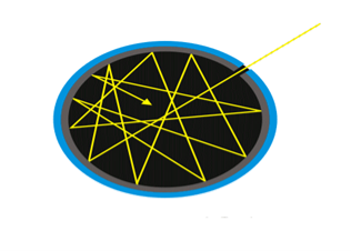
Figure1 : Black Body
The inside walls of a cavity radiator are rough and blackened so that any radiation that enters through a tiny hole in the cavity wall becomes trapped inside the cavity. At thermodynamic equilibrium (at temperature T), the cavity walls absorb exactly as much radiation as they emit. Furthermore, inside the cavity, the radiation entering the hole is balanced by the radiation leaving it. The emission spectrum of a blackbody can be obtained by analyzing the light radiating from the hole. Electromagnetic waves emitted by a blackbody are called blackbody radiation.
Spectral Distribution of energy in thermal radiation (Black Body radiation spectrum)
A good absorber of radiation is also a good emitter. Hence when a black body is heated it emits radiations. In practice a black body can be realized with the emission of Ultraviolet, Visible and infrared wavelengths on heating a body.
German physicists Lummer and Pringsheim studied the energy density as a function of wavelength for different temperatures of a black body using a spectrograph and a plot is made. This is called Black Body radiation spectrum.
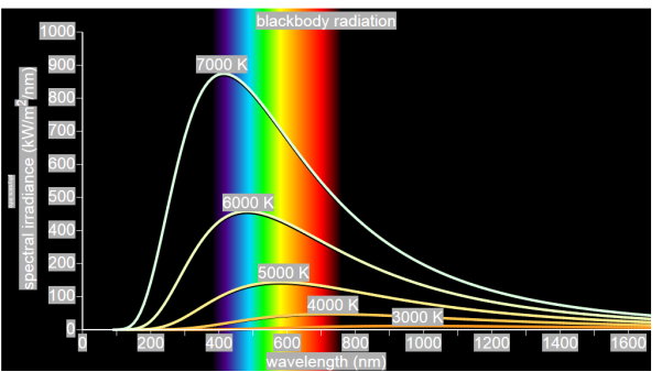
Figure 2: Black Body radiation spectrum
You can see the spectrum of a black body (and attempts to model that spectrum) in the above figure, for different temperatures. One needs simply to analyse the spectral distribution of the radiation coming out of the hole. The radiation emitted by a blackbody when hot is called blackbody radiation.
The intensity I(λ,T) of blackbody radiation depends on the wavelength λ of the emitted radiation and on the temperature T of the blackbody.
The function I(λ,T) is the power intensity that is radiated per unit wavelength.
In other words, it is the power radiated per unit area of the hole in a cavity radiator per unit wavelength. According to this definition, I(λ,T)dλ is the power per unit area that is emitted in the wavelength interval from λ to λ+dλ.
The intensity distribution among wavelengths of radiation emitted by cavities was studied experimentally at the end of the nineteenth century. Generally, radiation emitted by materials only approximately follows the blackbody radiation curve. However, spectra of common stars do follow the blackbody radiation curve very closely.
Experimental data about blackbody radiation was obtained for various objects. Following results obtained,
- At equilibrium, the radiation emitted has a well-defined, continuous energy distribution.
- To each frequency there corresponds an energy density which depends neither on the chemical composition of the object nor on its shape, but only on the temperature of the cavity’s walls.
- The energy density shows a pronounced maximum at a given frequency, which increases with temperature; that is, the peak of the radiation spectrum occurs at a frequency that is proportional to the temperature. This is the underlying reason behind the change in colour of a heated object as its temperature increases, notably from red to yellow to white.
It turned out that the explanation of the blackbody spectrum was not so easy. The problem was that nobody was able to come up with a theoretical explanation for the spectrum of light generated by the black body. Everything classical physics could come up with went wrong.
Key Takeaways
- A Body which is capable of absorbing almost all the radiations incident on it is called a black body.
- A perfectly black-body can absorb the entire radiations incident on it. Platinum black and Lamp black can absorb almost all the radiations incident on them.
- Emissive power of a black body is defined as the total energy radiated per second from the unit surface area of a black body maintained at certain temperature.
- Absorptive power of a black body is defined as the ratio of the total energy absorbed by the black body to the amount of radiant energy incident on it in a given time interval. The absorptive power of a perfectly black body is 1.
Derivation of Planck’s law
While Wien’s formula and the Rayleigh-Jeans Law could not explain the spectrum of a black body, Max Planck’s equation solved the problem by assuming that light was discrete.
The photoelectric effect demonstrates that light waves have particle properties and that the light quanta or photons of a particular frequency v each have energy hv. We need to reconcile this picture with the classical picture of electromagnetic waves in a box. In the classical picture, the energy associated with the waves is stored in the oscillating electric and magnetic fields.
We found it necessary to impose the constraint that only certain modes are permitted by the boundary conditions; the waves are constrained to fit into the box with whole numbers of half wavelengths in the x, y, z directions.
Now we have a further constraint. The quantisation of electromagnetic radiation means that the energy of a particular mode of frequency v cannot have any arbitrary value but only those energies which are multiples of hν, in other words the energy of the mode is E(ν) =nhv, where we associate n photons with this mode.
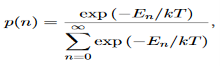
We now consider all the modes (and photons) to be in thermal equilibrium at temperature T. In order to establish equilibrium, there must be ways of exchanging energy between the modes (and photons) and this can occur through interactions with any particles or oscillators within the volume or with the walls of the enclosure. We now use the Boltzmann distribution to deter-mine the expected occupancy of the modes in thermal equilibrium. The probability that a single mode has energy En=nhv is given by the usual Boltzmann factor
 ……….(19)
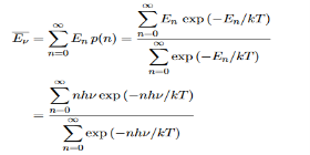
Where the denominator ensures that the total probability is unity, the usual normalisation procedure. In the language of photons, this is the probability that the state contains n photons of frequency ν. The mean energy of the mode of frequency ν is therefore
……….(20)
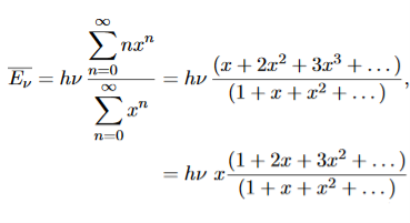
To simplify the calculation, let us substitute x=exp(−hν/kT). Then (20) becomes
 ……….(21)
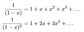
Now, we remember the following series expansions:
 ………….(22)
Hence, the mean energy of the mode is
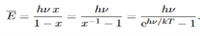 ………….(23)
This is the result we have been seeking. To find the classical limit, we allow the energy quanta hν to tend to zero.
Expanding ehν/kT−1 for small values of hν/kT,
ehν/kT−1 = 1 +hν/kT+ !(hν/kT)2+···−1 ………….(24)
Thus, for small values of hν/kT, ehν/kT−1 =hν/kT.
And also
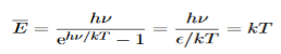 …………….(25)
Thus, if we take the classical limit, we recover exactly the expression for the average energy of a harmonic oscillator in thermal equilibrium,  =kT. We can now complete the determination of Planck’s radiation formula.
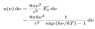
We have already shown that the number of modes in the frequency interval ν to ν+dν is (8πν2/c3) dν per unit volume. The Planck distribution in terms of the energy density of radiation per unit frequency interval
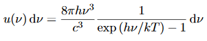
The energy density of radiation in this frequency range is
 ………….(26)
This is the Planck distribution function.
Key Takeaways
While Wien’s formula and the Rayleigh-Jeans Law could not explain the spectrum of a black body, Max Planck’s equation solved the problem by assuming that light was discrete.
- The photoelectric effect demonstrates that light waves have particle properties and that the light quanta or photons of a particular frequency v each have energy hv.
- The Planck distribution in terms of the energy density of radiation per unit frequency interval

In 1887 Hertz discovered the photoelectric effect. The photoelectric effect confirms the concept of energy quantization of light.
Photoelectric Effect: when a metal is irradiated with light, electrons may get emitted.
Electrons were observed to be ejected from metals when irradiated with light as shown in Figure 3(a).
Moreover, the following experimental laws were discovered prior to 1905:
- If the frequency of the incident radiation is smaller than the metal’s threshold frequency no electron can be emitted regardless of the radiation’s intensity.
- No matter how low the intensity of the incident radiation, electrons will be ejected instantly the moment the frequency of the radiation exceeds the threshold frequency.
- At any frequency above, the number of electrons ejected increases with the intensity of the light but does not depend on the light’s frequency.
- The kinetic energy of the ejected electrons depends on the frequency but not on the intensity of the beam; the kinetic energy of the ejected electron increases linearly with the incident frequency.
In 1905 Einstein gave a theoretical explanation for the dependence of photoelectric emission on the frequency of the incident radiation. He assumed that light is made of corpuscles each carrying an energy h ν, called photons. When a beam of light of frequency ν is incident on a metal, each photon transmits all its energy hν to an electron near the surface; in the process, the photon is entirely absorbed by the electron. The electron will thus absorb energy only in quanta of energy h ν , irrespective of the intensity of the incident radiation. If hν is larger than the metal’s work function W
Work function is defined as the minimum energy required to eject an electron from the metal.
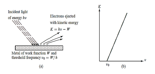
Figure 3: (a) Photoelectric effect (b) Kinetic energy K of the electron leaving the metal when irradiated with a light of frequency ν ; when ν < ν0 no electron is ejected from the metal regardless of the intensity of the radiation.
Hence no electron can be emitted from the metal’s surface unless h ν >W:
h ν =W +K
Where K represents the kinetic energy of the electron leaving the material.
The above equation gives the proper explanation to the experimental observation that the kinetic energy of the ejected electron increases linearly with the incident frequency ν, as shown in Figure 3(b):
K = h ν - W = h(ν -ν0)
Where ν0 =W/h is called the threshold or cut off frequency of the metal. Moreover, this relation shows clearly why no electron can be ejected from the metal unless ν > ν0 since the kinetic energy cannot be negative, the photoelectric effect cannot occur when ν < ν0 regardless of the intensity of the radiation. The ejected electrons acquire their kinetic energy from the excess energy h(ν -ν0)supplied by the incident radiation.
The kinetic energy of the emitted electrons can be experimentally determined as follows.
The set up consists of the photoelectric metal (cathode) that is placed next to an anode inside an evacuated glass tube. When light strikes the cathode’s surface, the electrons ejected will be attracted to the anode, thereby generating a photoelectric current.
The magnitude of the photoelectric current thus generated is proportional to the intensity of the incident radiation, yet the speed of the electrons does not depend on the radiation’s intensity, but on its frequency.
To measure the kinetic energy of the electrons, we simply need to use a varying voltage source and reverse the terminals. When the potential V across the tube is reversed, the liberated electrons will be prevented from reaching the anode; only those electrons with kinetic energy larger than e will make it to the negative plate and contribute to the current.
We vary V until it reaches a value Vs called the stopping potential, at which all of the electrons, even the most energetic ones, will be turned back before reaching the collector; hence the flow of photoelectric current ceases completely.
The stopping potential Vs is connected to the electrons’ kinetic energy by
e =
=  mev2 = K
Thus, the relation becomes
e == h ν - W
Or can be written as
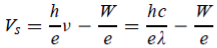
The shape of the plot of Vs against frequency is a straight line, much like Figure 3(b) with the slope now given by h/e. This shows that the stopping potential depends linearly on the frequency of the incident radiation.
Key Takeaways
- Photoelectric Effect: when a metal is irradiated with light, electrons may get emitted.
- No electron can be ejected from the metal unless ν > ν0 since the kinetic energy cannot be negative, the photoelectric effect cannot occur when ν < ν0 regardless of the intensity of the radiation.
- The magnitude of the photoelectric current thus generated is proportional to the intensity of the incident radiation, yet the speed of the electrons does not depend on the radiation’s intensity, but on its frequency.
- The stopping potential depends linearly on the frequency of the incident radiation.
In his 1923 experiment, Compton provided the most conclusive confirmation of the particle aspect of radiation.
By scattering X-rays off free electrons, he found that the wavelength of the scattered radiation is larger than the wavelength of the incident radiation. This can be explained only by assuming that the X-ray photons behave like particles.
According to classical physics, the incident and scattered radiation should have the same wavelength.
Also, we know that the energy of the X-ray radiation is too high to be absorbed by a free electron therefore the incident X-ray would then provide an oscillatory electric field which sets the electron into oscillatory motion, hence making it radiate light with the same wavelength but with an intensity I that depends on the intensity of the incident radiation I0
But neither of these two predictions of classical physics is compatible with experiment.
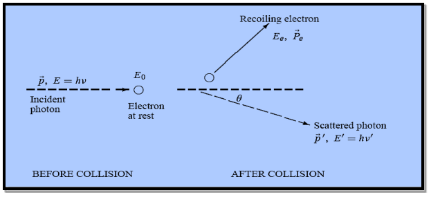
Figure 4: Elastic scattering of a photon from a free electron
By experiment Compton reveals that the wavelength of the scattered X-radiation increases by an amount  , called the wavelength shift and that
  depends not on the intensity of the incident radiation, but only on the scattering angle.
Compton succeeded in explaining his experimental results only after treating the incident radiation as a stream of particles—photons—colliding elastically with individual electrons.
Here we will discuss the elastic scattering of a photon from a free-electron as shown in the figure. Consider that the incident photon, of energy E =hν and momentum p = hν /c, collides with an electron that is initially at rest. If the photon scatters with a momentum at an angle θ while the electron recoils with a momentum
  the conservation of linear momentum yields
 =
=  +
+  …………(1)
Which leads
 = (
= ( -
-  )2 =
)2 =  +
+  -2pp’cosθ =
  (
(  +
+  -2νν’cosθ) ………. . (2)
Energy Conservation
The energies of the electron before and after the collision are given, respectively, by
E0 =mec2 ………. . (3)

Since the energies of the incident and scattered photons are given by E = hν and E0 = hν’, respectively, conservation of energy dictates that
E + E0 = E’ + Ee ………. . (4)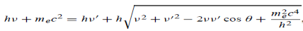 ………. . (5)
Which leads to
 ………. . (6)
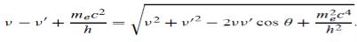
Squaring both sides of (5) and simplifying, we get
Hence wavelength shift is given by

Where λC = h/mec = 2. 426 x 10-12 m is called the Compton wavelength of the electron.
This relation connects the initial and final wavelengths to the scattering angle.
Compton’s experimental observation:
- The wavelength shift of the X-rays depends only on the angle at which they are scattered and not on the frequency (or wavelength) of the incident photons.
- The Compton Effect confirms that photons behave like particles. They collide with electrons like material particles.
Example
High energy photons are scattered from electrons initially at rest. Assume the photons are backscattered and their energies are much larger than the electron’s rest-mass energy, E = mec2.
(a) Calculate the wavelength shift.
(b) Show that the energy of the scattered photons is half the rest mass energy of the electron, regardless of the energy of the incident photons.
(c) Calculate the electron’s recoil kinetic energy if the energy of the incident photons is 150 MeV.
Solution:
(a) In the case where the photons backscatter i. e. θ = π
The wavelength shift becomes
 =
=  -
-  = 2
= 2 c sin2θ = 2
 c sin2 π = 2
 c = 2 x 2. 426 x 10-12 m =4. 86 x 10-12 m
(b) Since the energy of the scattered photons E’ is related to the wavelength  by E =hc /

Where E = hc/  is the energy of the incident photons. If E = mec2 we can approximate

(c) If E = 150 MeV, the kinetic energy of the recoiling electrons can be obtained from the conservation of energy
Ke = E – E’  150 – 0. 25 =14. 75 MeV
Example
X-rays with an energy of 300 keV undergo Compton scattering with a target. If the scattered X-rays are detected at 30° relative to the incident X-rays, determine the Compton shift at this angle, the energy of the scattered X-ray, and the energy of the recoiling electron.
Solution:
The Compton shift
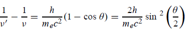
When it is scattered through an angle θ by an electron: λ′−λ= λe(1−cosθ)
We know Compton wavelength of the electron λe= h/mec= 2. 43 pm
me mass of the electron = 511 keV/c2
θ = 30°
Compton shift is
λ′−λ= λe(1−cosθ) = 2. 426 x 10-12 m (1−cos30◦. ) = 0. 325 pm
The energy E′ of the scattered photon is E′=hc/ λ′
And λ=hc/E
E=300 keV is the wavelength of the incoming photon. It follows that E′= 278 keV. By conservation of energy, the energy lost by the photon in the collision is converted into kinetic energy K of the recoiling electrons K= 22 keV
Key Takeaways
- Compton reveal that the wavelength of the scattered X-radiation increases by an amount
 , called the wavelength shift, and that
- It depends not on the intensity of the incident radiation, but only on the scattering angle.
- Compton succeeded in explaining his experimental results only after treating the incident radiation as a stream of particles—photons—colliding elastically with individual electrons.
- Hence wavelength shift is given by
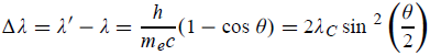
- Where λC = h/mec = 2.426 x 10⁻¹² m is called the Compton wavelength of the electron.
Einstein Equation
Quantum mechanics began with two deceptively simple formulas
E= and p= h/λ
These are the Einstein and de Broglie relations, respectively.
De Broglie Hypothesis of Matter Waves
As we know in the Photoelectric Effect, the Compton Effect, and the pair production effect—radiation exhibits particle-like characteristics in addition to its wave nature. In 1923 de Broglie took things even further by suggesting that this wave–particle duality is not restricted to radiation, but must be universal.
In 1923, the French physicist Louis Victor de Broglie (1892-1987) put forward the bold hypothesis that moving particles of matter should display wave-like properties under suitable conditions.
All material particles should also display dual wave–particle behaviour. That is, the wave–particle duality present in light must also occur in matter.
So, starting from the momentum of a photon p = hν/c = h/λ.
We can generalize this relation to any material particle with nonzero rest mass. Each material particle of momentum  behaves as a group of waves (matter waves) whose wavelength λ and wave vector
  are governed by the speed and mass of the particle. De Broglie proposed that the wave length λ associated with a particle of momentum p is given as where m is the mass of the particle and v its speed.
λ =  =
= …….(1)
  =
=  …….(2)
Where ℏ = h/2π. The expression known as the de Broglie relation connects the momentum of a particle with the wavelength and wave vector of the wave corresponding to this particle. The wavelength λ of the matter wave is called de Broglie wavelength. The dual aspect of matter is evident in the de Broglie relation.
λ is the attribute of a wave while on the right hand side the momentum p is a typical attribute of a particle. Planck’s constant h relates the two attributes. Equation (1) for a material particle is basically a hypothesis whose validity can be tested only by experiment.
However, it is interesting to see that it is satisfied also by a photon. For a photon, as we have seen, p = hν/c.
Therefore
 =
=  = λ
= λ
Matter waves: According to De-Broglie, a wave is associated with each moving particle which is called matter waves.
That is, the wave–particle duality present in light must also occur in matter. So, starting from the momentum of a photon p = h ν /c = h/λ, we can generalize this relation to any material particle with nonzero rest mass: each material particle of momentum  behaves as a group of waves (matter waves) whose wavelength λ and wave vector
 are governed by the speed and mass of the particle.
λ = 
 =
= 
Wave has wavelength λ here h is Planck's constant and p is the momentum of the moving particle.
We have seen that microscopic particles, such as electrons, display wave behaviour. What about macroscopic objects? Do they also display wave features? They surely do. Although macroscopic material particles display wave properties, the corresponding wavelengths are too small to detect; being very massive, macroscopic objects have extremely small wavelengths.
At the microscopic level, however, the waves associated with material particles are of the same size or exceed the size of the system. Microscopic particles therefore exhibit clearly noticeable wave-like aspects.
The general rule is: whenever the de Broglie wavelength of an object is in the range of, or exceeds, its size, the wave nature of the object is detectable and hence cannot be neglected.
But if its de Broglie wavelength is much too small compared to its size, the wave behaviour of this object is undetectable.
For a quantitative illustration of this general rule, let us calculate in the following example the wavelengths corresponding to two particles, one microscopic (electron) and the other macroscopic (ball).
Key Takeaways
- Quantum mechanics began with two deceptively simple formula E=
 and p= h/λ. These are the Einstein and de Broglie relations respectively.
 - De Broglie (1892-1987) put forward the bold hypothesis that moving particles of matter should display wave-like properties under suitable conditions.
- All material particles should also display dual wave–particle behaviour. That is, the wave–particle duality present in light must also occur in matter.
- The expressions known as the de Broglie relation
λ =  =
=
 =
= 
Where ℏ = h/2π. The expression known as the de Broglie relation
In this experiment, Davisson and Germer scattered a 54 eV monoenergetic beam of electrons from a nickel (Ni) crystal. The electron source and detector were symmetrically located with respect to the crystal’s normal, as shown in figure this is similar to the Bragg setup for X-ray diffraction by a grating. What Davisson and Germer found was that, although the electrons are scattered in all directions from the crystal, the intensity was a minimum at θ = 35°
WAVE ASPECT OF PARTICLES
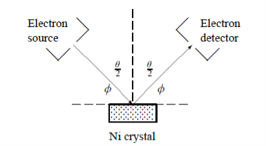
Figure 5: Davisson–Germer experiment: electrons strike the crystal’s surface at an angle ϕ
The detector, symmetrically located from the electron source, measures the number of electrons scattered at an angle θ, where θ is the angle between the incident and scattered electron beams.
It is maximum at θ = 50°; that is, the bulk of the electrons scatter only in well-specified directions. They showed that the pattern continued even when the intensity of the beam was so low that the incident electrons were sent one at a time. This can only result from a constructive interference of the scattered electrons. The reflected electrons formed diffraction patterns that were identical
With Bragg’s X-ray diffraction by a grating instead of the diffuse distribution pattern.
In fact, the intensity maximum of the scattered electrons in the Davisson–Germer experiment corresponds to the first maximum (n = 1) of the Bragg formula,
nλ = 2d sin ϕ
Where d is the spacing between the Bragg planes
ϕ is the angle between the incident ray and the crystal’s reflecting planes
θ is the angle between the incident and scattered beams
d is given in terms of the separation D between successive atomic layers in the crystal by d = D sin θ
For an Ni crystal, we have d = 0.091 nm, since D = 0.215 nm. Since only one maximum is seen at θ = 50° for a mono-energetic beam of electrons of kinetic energy 54 eV, and since 2ϕ +  = π and hence sin ϕ = cos(θ /2) from figure.
We can obtain the wavelength associated with the scattered electrons:
λ =  sin ϕ =
  cos
cos  θ =
θ =  cos 25° = 0.165 nm
Now using results from de Broglie’s relation we will calculate the numerical value of λ. Since the kinetic energy of the electrons is K = 54 eV, and the momentum is p = with mec2 = 0.511 MeV.
Where mec2 is the rest mass energy of the electron and hc  197.33 eV nm, we can show that the de Broglie wavelength is
λ =  =
=
 = 0.167 nm
This is in excellent agreement with the experimental value.
We have seen that the scattered electrons in the Davisson–Germer experiment produced interference fringes that were identical to those of Bragg’s X-ray diffraction. Since the Bragg formula provided an accurate prediction of the electrons’ interference fringes, the motion of an electron of momentum must be described by means of a plane wave
ψ(r, t) =Aei(k·r−ωt) = Aei(p·r−Et)/
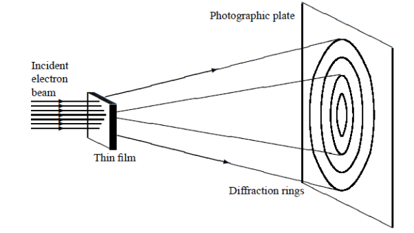
Figure 6: Davisson–Germer experiment
Key Takeaways
- Davisson and Germer found was that, although the electrons are scattered in all directions from the crystal, the intensity was a minimum at θ = 35°
- We have seen that the scattered electrons in the Davisson–Germer experiment produced interference fringes that were identical to those of Bragg’s X-ray diffraction.
- Kinetic energy of the electrons is K = 54 eV, and the momentum is p =
 with mec2 = 0.511 MeV.Where mec2 is the rest mass energy of the electron and hc
  197.33 eV nm,
 - The de Broglie wavelength is
λ =  =
=
 = 0.167 nm
According to classical physics, given the initial conditions and the forces acting on a system, the future behaviour (unique path) of this physical system can be determined exactly. That is, if the initial coordinates , velocity
  , and all the forces acting on the particle are known, the position
  , and velocity
  are uniquely determined by means of Newton’s second law. So by Classical physics it can be easily derived.
Does this hold for the microphysical world?
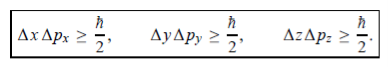
Since a particle is represented within the context of quantum mechanics by means of a wave function corresponding to the particle’s wave, and since wave functions cannot be localized, then a microscopic particle is somewhat spread over space and, unlike classical particles, cannot be localized in space. In addition, we have seen in the double-slit experiment that it is impossible to determine the slit that the electron went through without disturbing it. The classical concepts of exact position, exact momentum, and unique path of a particle therefore make no sense at the microscopic scale. This is the essence of Heisenberg’s uncertainty principle.
In its original form, Heisenberg’s uncertainty principle states that: If the x-component of the momentum of a particle is measured with an uncertainty ∆px, then its x-position cannot, at the same time, be measured more accurately than ∆x = ℏ/(2∆px). The three-dimensional form of the uncertainty relations for position and momentum can be written as follows:

This principle indicates that, although it is possible to measure the momentum or position of a particle accurately, it is not possible to measure these two observables simultaneously to an arbitrary accuracy. That is, we cannot localize a microscopic particle without giving to it a rather large momentum.
We cannot measure the position without disturbing it; there is no way to carry out such a measurement passively as it is bound to change the momentum.
To understand this, consider measuring the position of a macroscopic object (you can consider a car) and the position of a microscopic system (you can consider an electron in an atom). On the one hand, to locate the position of a macroscopic object, you need simply to observe it; the light that strikes it and gets reflected to the detector (your eyes or a measuring device) can in no measurable way affect the motion of the object.
On the other hand, to measure the position of an electron in an atom, you must use radiation of very short wavelength (the size of the atom). The energy of this radiation is high enough to change tremendously the momentum of the electron; the mere observation of the electron affects its motion so much that it can knock it entirely out of its orbit.
It is therefore impossible to determine the position and the momentum simultaneously to arbitrary accuracy. If a particle were localized, its wave function would become zero everywhere else and its wave would then have a very short wavelength. According to de Broglie’s relation p = ℏ /λ,
Time Energy Uncertainty Relation
The momentum of this particle will be rather high. Formally, this means that if a particle is accurately localized (i.e., ∆x  0), there will be total uncertainty about its momentum (i.e., ∆px
  ∞).
∞).
Since all quantum phenomena are described by waves, we have no choice but to accept limits on our ability to measure simultaneously any two complementary variables.
Heisenberg’s uncertainty principle can be generalized to any pair of complementary, or canonically conjugate, dynamical variables: it is impossible to devise an experiment that can measure simultaneously two complementary variables to arbitrary accuracy .If this were ever achieved, the theory of quantum mechanics would collapse.
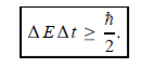
Energy and time, for instance, form a pair of complementary variables. Their simultaneous measurement must obey the time–energy uncertainty relation:

This relation states that if we make two measurements of the energy of a system and if these measurements are separated by a time interval ∆t, the measured energies will differ by an amount ∆E which can in no way be smaller than ℏ /∆t. If the time interval between the two measurements is large, the energy difference will be small. This can be attributed to the fact that, when the first measurement is carried out, the system becomes perturbed and it takes it a long time to return to its initial, unperturbed state. This expression is particularly useful in the study of decay processes, for it specifies the relationship between the mean lifetime and the energy width of the excited states.
In contrast to classical physics, quantum mechanics is a completely indeterministic theory. Asking about the position or momentum of an electron, one cannot get a definite answer; only a probabilistic answer is possible.
According to the uncertainty principle, if the position of a quantum system is well defined its momentum will be totally undefined.
APPLICATION OF UNCERTAINTY PRINCIPLE
The Heisenberg uncertainty principle based on quantum physics explains a number of facts which could not be explained by classical physics.
- Non-existence of electrons in the nucleus or Non-confinement of electron in the nucleus)
One of the applications is to prove that electron cannot exist inside the nucleus.
But to prove it, let us assume that electrons exist in the nucleus.
As the radius of the nucleus in approximately 10-14m. If electron is to exist inside the nucleus, then uncertainty in the position of the electron is given by
According to uncertainty principle
∆x ∆p =h/2π
Thus ∆p=h/2π∆x
Or ∆p=6.62 x10⁻³⁴/2 x 3.14 x 10-14
Or ∆p=1.05 x 10⁻²⁰ kg m/ sec
If this is p the uncertainty in the momentum of electron then the momentum of electron should be at least of this order that is p=1.05*10-20 kg m/sec.
An electron having this much high momentum must have a velocity comparable to the velocity of light. Thus, its energy should be calculated by the following relativistic formula
E = 
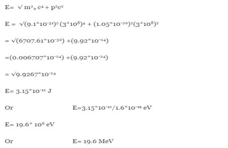
Therefore, if the electron exists in the nucleus, it should have an energy of the order of 19.6 MeV.
However, it is observed that beta-particles (electrons) ejected from the nucleus during b – decay have energies of approximately 3 Me V, which is quite different from the calculated value of 19.6 MeV.
Another reason that electron cannot exist inside the nucleus is that experimental results show that no electron or particle in the atom possess energy greater than 4 MeV.
Therefore, it is confirmed that electrons do not exist inside the nucleus.
2. Ground State Energy of A Harmonic Oscillator or Calculation of zero point energy
Zero-point energy (ZPE) is the lowest possible energy that a quantum mechanical system may have. Unlike in classical mechanics, quantum systems constantly fluctuate in their lowest energy state as described by the Heisenberg uncertainty principle. As well as atoms and molecules, the empty space of the vacuum has these properties. According to quantum field theory, the universe can be thought of not as isolated particles but continuous fluctuating fields: matter fields, whose quanta are fermions and force fields, whose quanta are bosons. All these fields have zero-point energy.
The minimum energy of a system at o k (zero kelvin) is called zero point energy.
Consider a particle which is confined to move under the influence of potential of dimensions a. Since the particle may be present anywhere in these dimensions, so uncertainty in position
∆x = a/2 (half the diameter).
According to uncertainty principle
∆x∆px = ℏ/2
Or
Thus ∆px= ℏ /2∆x
∆px= ℏ /2a/2 = ℏ /a
Uncertainty in momentum of particle along x-axis is
∆px= ℏ /a
Assuming the momentum of particle to be at least equal to uncertainty in it, the lowest possible value of K.E. Of particle is given by
K.E. =  =
=  =
=
Where m is the mass of the particle.
Energy even at O K is given by the above equation. This minimum energy is called the zero-point energy.
This implies that even at zero kelvin, the particle is never at rest. If it is so, then ∆pX = 0, which is not possible. [It gives ∆x = ∞]
3. Existence of proton, neutron and alpha particles within the nucleus.
We know that the rest mass of the protons and neutron is of the order of
The corresponding value of kinetic energy of a neutron or a proton is
E =  =
=  =8.33 x 10⁻¹⁵J =
 eV
eV
 52.05 keV
Since the rest mass of the a-particle is nearly four times the proton mass, therefore the alpha particle should have a minimum kinetic energy of one fourth of 52.05 keV, or about 13 keV. Since the energy carried by the protons or neutrons emitted by the nuclei are greater than 52 keV and for a-particle more than 13 keV, these particles can exist in the nuclei.
4. Size of Elementary cell in Phase space
We have studied in our previous class that state of a microsystem is defined by six variables – three are due to position and three due to momentum.
Hence, a system of N particles needs 6 N variables
If ∆ x and ∆px be the uncertainly in position and in momentum measurements then
∆ x ∆ px =  ;
;
Similarly ∆ y ∆ py =  ,
,
And ∆ z ∆ pz =  ,
,
Multiplying these three equations, we get
∆ x ∆ y ∆ z ∆ px ∆ py ∆ pz = (  )3 in the units (J3 S3).
The above product is called the volume of elementary cell in phase space.
So, volume of an elementary cell in phase space  10-101 units, (for quantum statistics) being
 .
.
5. Accurate limit of frequency of radiation emitted by an atom
Consider the radiation emitted from an excited atom. The energy of this atom will decrease when it emits one or more photons of characteristic frequency.
The average period between excitation of the atom and the release of energy is about 10-8 seconds.
Thus, uncertainly in energy is
∆ E 

Or ∆ E 
 J
J
Or ∆ E  5.3 x 10⁻²⁷ J
Frequency of light is uncertain by
∆ ν =  =
=  Hz
Hz  0.8 x 10⁷ Hz
As a result, the radiation from an excited atom does not have the noted precise frequency new ν - ∆ ν and ν + ∆ ν.
Key Takeaways
- Heisenberg’s uncertainty principle states that: If the x-component of the momentum of a particle is measured with an uncertainty ∆px, then its x-position cannot, at the same time, be measured more accurately than ∆x = ℏ/(2∆px).
- The three-dimensional form of the uncertainty relations for position and momentum can be written as follows:
- This principle indicates that, although it is possible to measure the momentum or position of a particle accurately, it is not possible to measure these two observables simultaneously to an arbitrary accuracy. That is, we cannot localize a microscopic particle without giving to it a rather large momentum.
- Energy and time, for instance, form a pair of complementary variables. Their simultaneous measurement must obey the time–energy uncertainty relation:
- Electron cannot exist inside the nucleus because experimental results show that no electron or particle in the atom possess energy greater than 4 MeV.
- Zero-point energy (ZPE) is the lowest possible energy that a quantum mechanical system may have. Unlike in classical mechanics, quantum systems constantly fluctuate in their lowest energy state as described by the Heisenberg uncertainty principle.
- Heisenberg uncertainty principle proves proton, neutron and alpha particles exists within the nucleus.
- Size of Elementary cell in Phase space is given by Heisenberg uncertainty principle
- Frequency of light is uncertain by
∆ ν =  =
=  Hz
Hz  0.8 x 10⁷ Hz
Quantum theory and determinism usually do not go together. A natural combination is quantum theory and randomness. Indeed, when in the end of 19th century physics seemed to be close to provide a very good deterministic explanation of all observed phenomena, Lord Kelvin identified “two clouds” on “the beauty and clear-ness of the dynamical theory”. One of this “clouds” was the quantum theory which brought a consensus that there is randomness in physics. Recently we even “certify” randomness using quantum experiments
The quantum theory of the wave function of the Universe is a very successful deterministic theory fully consistent with our experimental evidence. However, it requires accepting that the world we experience is only part of the reality and there are numerous parallel worlds. The existence of parallel worlds allows us to have a clear deterministic and local physical theory.
Wave Function
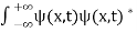
The wave function, at a particular time, contains all the information that anybody at that time can have about the particle. But the wave function itself has no physical interpretation. It is not measurable. However, the square of the absolute value of the wave function has a physical interpretation. We interpret |ψ(x,t)|2 as a probability density, a probability per unit length of finding the particle at a time t at position x.
The wave function ψ associated with a moving particle is not an observable quantity and does not have any direct physical meaning. It is a complex quantity. The complex wave function can be represented as
ψ(x, y, z, t) = a + ib
And its complex conjugate as
ψ*(x, y, z, t) = a – ib.
The product of wave function and its complex conjugate is
ψ(x, y, z, t)ψ*(x, y, z, t) = (a + ib) (a – ib) = a2 + b2
a2 + b2 is a real quantity.
However, this can represent the probability density of locating the particle at a place in a given instant of time.
The positive square root of ψ(x, y, z, t) ψ*(x, y, z, t) is represented as |ψ(x, y, z, t)|, called the modulus of ψ. The quantity |ψ(x, y, z, t)|2 is called the probability. This interpretation is possible because the product of a complex number with its complex conjugate is a real, non-negative number.
We should be able to find the particle somewhere, we should only find it at one place at a particular instant, and the total probability of finding it anywhere should be one.
For the probability interpretation to make sense, the wave function must satisfy certain conditions.
- The wave function must be single valued at each point.
- The probability of finding the particle at time t in an interval ∆x must be some number between 0 and 1.
- ψ must be finite everywhere.
- ψ must be continuous everywhere and
 must also be continuous everywhere except where V(x) is infinite.
 - ψ (x) must vanish ψ
 0 as x
 .
. - The wave function should satisfy the normalization condition. Normalization condition of a wave function ψ is mathematical statement of existence of the particle somewhere. So that if we sum up all possible values ∑|ψ(xi,t)|2∆xi we must obtain 1. The total probability of finding the particle anywhere must be one. Normalization condition is given as
 dx =1
dx =1
Only wave function with all these properties can yield physically meaningful result.
Physical significance of wave function
- The wave function ‘Ѱ’ has no physical meaning. It is a complex quantity representing the variation of a matter wave.
- The wave function Ѱ(r,t) describes the position of particle with respect to time .
- It can be considered as ‘probability amplitude’ since it is used to find the location of the particle.
- The square of the wave function gives the probability density of the particle which is represented by the wave function itself.
- More the value of probability density, more likely to find the particle in that region.
The Schrodinger equation also known as Schrodinger’s wave equation is a partial differential equation that describes the dynamics of quantum mechanical systems by the wave function. The trajectory, the positioning, and the energy of these systems can be retrieved by solving the Schrodinger equation.
All of the information for a subatomic particle is encoded within a wave function. The wave function will satisfy and can be solved by using the Schrodinger equation. The Schrodinger equation is one of the fundamental axioms that are introduced in undergraduate physics.
Statistical Interpretation
It is not possible to measure all properties of a quantum system precisely. Max Born suggested that the wave function was related to the probability that an observable has a specific value.
In any physical wave if ‘A’ is the amplitude of the wave, then the energy density i.e., energy per unit volume is equal to ‘A2’. Similar interpretation can be made in case of mater wave also. In matter wave, if ‘Ψ ‘is the wave function of matter waves at any point in space, then the particle density at that point may be taken as proportional to ‘Ψ2’ . Thus Ψ2 is a measure of particle density.
According to Max Born ΨΨ*=Ψ2 gives the probability of finding the particle in the state ‘Ψ’. i.e., ‘Ψ2’ is a measure of probability density. The probability of finding the particle in a volume (dv=dxdydz) is given by
 =
= 
Since the particle has to be present somewhere, total probability of finding the particle somewhere is unity i.e., particle is certainly to be found somewhere in space. i.e.
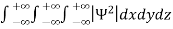 =1
=1
Or  =1
=1
This condition is called Normalization condition. A wave function which satisfies this condition is known as normalized wave function.
The wave function, at a particular time, contains all the information that anybody at that time can have about the particle. But the wave function itself has no physical interpretation. It is not measurable. However, the square of the absolute value of the wave function has a physical interpretation. We interpret |ψ(x,t)|2 as a probability density, a probability per unit length of finding the particle at a time t at position x.
Key Takeaways
- The wave function, at a particular time, contains all the information that anybody at that time can have about the particle. But the wave function itself has no physical interpretation. It is not measurable.
- The wave function must be single valued at each point. The probability of finding the particle at time t in an interval ∆x must be some number between 0 and 1. ψ must be finite everywhere.
- According to Max Born ΨΨ*=Ψ2 gives the probability of finding the particle in the state ‘Ψ’. i.e., ‘Ψ2’ is a measure of probability density. The probability of finding the particle in a volume (dv=dxdydz) is given by
 =
= 
Schrodinger wave equation, is the fundamental equation of quantum mechanics, same as the second law of motion is the fundamental equation of classical mechanics. This equation has been derived by Schrodinger in 1925 using the concept of wave function on the basis of de-Broglie wave and plank’s quantum theory.
Let us consider a particle of mass m and classically the energy of a particle is the sum of the kinetic and potential energies. We will assume that the potential is a function of only x.
So We have
E= K+V = mv2+V(x) =
 +V(x) ……….. (1)
By de Broglie’s relation we know that all particles can be represented as waves with frequency ω and wave number k, and that E= ℏω and p= ℏk.
Using this equation (1) for the energy will become
ℏω =  + V(x) ……….. (2)
A wave with frequency ω and wave number k can be written as usual as
ψ(x, t) =Aei(kx−ωt) ……….. (3)
The above equation is for one dimensional and for three dimensional we can write it as
ψ(r, t) =Aei(k·r−ωt) ……….. (4)
But here we will stick to one dimension only.
 =−iωψ ⇒ ωψ=
 ……….. (5)
 =−k2ψ ⇒ k2ψ = -
  ……….. (6)
If we multiply the energy equation in Eq. (2) by ψ, and using(5) and (6) , we obtain
ℏ(ωψ) =  ψ+ V(x) ψ ⇒
  = -
= - 
 + V(x) ψ ……….. (7)
This is the time-dependent Schrodinger equation.
If we put the x and t in above equation then equation (7) takes the form as given below
 = -
= - 
 + V(x) ψ(x,t) ……….. (8)
In 3-D, the x dependence turns into dependence on all three coordinates (x, y, z) and the  term becomes ∇2ψ.
The term |ψ(x)|2 gives the probability of finding the particle at position x.
Let us again take it as simply a mathematical equation, then it’s just another wave equation. However We already know the solution as we used this function ψ(x, t) =Aei(kx−ωt) to produce Equations (5), (6) and (7)
But let’s pretend that we don’t know this, and let’s solve the Schrodinger equation as if we were given to us. As always, we will guess an exponential solution by looking at exponential behaviour in the time coordinate, our guess is ψ(x, t) =e−iωtf(x) putting this into Equation (7) and cancelling the e−iωt yields
 = -
= - 
 + V(x) f(x) ……….. (9)
We already know that E= . However ψ(x, t) is general convention to also use the letter ψ to denote the spatial part. So we will now replace f(x) with ψ(x)
Eψ = - 
 + V(x) ψ ……….. (10)
This is called the time-independent Schrodinger equation.
Key Takeaways
- Schrodinger wave equation, is the fundamental equation of quantum mechanics
- The time-dependent Schrodinger equation is given by
⇒  = -
= - 
 + V(x) ψ
- The time-independent Schrodinger equation is given by
Eψ = - 
 + V(x) ψ
Let us consider a particle of mass ‘m’ in a deep well restricted to move in a one dimension (say x). Let us assume that the particle is free inside the well except during collision with walls from which it rebounds elastically.
The potential function is expressed as
V= 0 for 0 ………. (1)
V=  for x <0, x>L ………. (2)
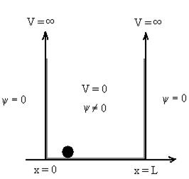
Figure 7: Particle in deep potential well
The probability of finding the particle outside the well is zero (i.e. Ѱ =0)
Inside the well, the Schrödinger wave equation is written as
 ψ +
ψ + E ψ =0 …………….(2)
Substituting  E = k2 …………….(3)
Writing the SWE for 1-D we get
 + k2 ψ =0 …………….(4)
The general equation of above equation may be expressed as
ψ = Asin (kx + ϕ) …………….(5)
Where A and ϕ are constants to be determined by boundary conditions
Condition I: We have ψ = 0 at x = 0, therefore from equation
0 = A sinϕ
As A  then sinϕ =0 or ϕ=0 …………….(6)
Condition II: Further ψ = 0 at x = L, and ϕ=0 , therefore from equation (5)
0 = Asin kL
As A  then sinkL =0 or kL=nπ
k =  …………….(7)
Where n= 1,2,3,4………
Substituting the value of k from (7) to (3)
 )2 =
)2 =  E
E
This gives energy of level
En =  n=1,2,3,4…so on …………….(8)
From equation En is the energy value (Eigen Value) of the particle in a well.
It is clear that the energy values of the particle in well are discrete not continuous.
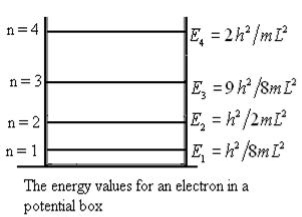
Figure 8: The energy values for an electron in a potential box
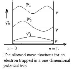
Using (6) and (7) equation (5) becomes, the corresponding wave functions will be
ψ = ψn = Asin …………….(9)
The probability density
|ψ(x,t)|2 = ψ ψ*
|ψ(x,t)|2 = A2sin2 …………….(10)
The probability density is zero at x = 0 and x = L. Since the particle is always within the well
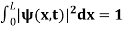 …………….(11)
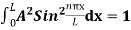
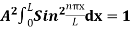
 =1
=1
A = 
Substituting A in equation (9) we get
ψ = ψn =  sin
sin n=1,2,3,4….. …………….(12)
The above equation (12) is normalized wave function or Eigen function belonging to energy value En
 F
F
Figure 9: Wave function for Particle
Key Takeaways
- It is assume that the particle is free inside the well except during collision with walls from which it rebounds elastically.
- The probability of finding the particle outside the well is zero (i.e. Ѱ =0)
- The energy values of the particle in well are discrete not continuous and Energy of level is given by
- En =
 n=1,2,3,4…so on
 - The probability density is given by
- |ψ(x,t)|2 = A2sin2

References Books
- Richard Robinett, Quantum Mechanics
- Quantum Mechanics Concepts & Applications -- Nouredine Zettili
- Introduction to Quantum Mechanics -- David J Griffiths
- Quantum Physics -- H.C.Verma


