UNIT 2: CALCULUS
2.1 Rolle’s theorem and Mean value theorems
Statement:
Suppose f(x) is continuous on  , differentiable on (a,b) and f(a) = f(b) .then there exists some point
  such that
Proof:
When proving a theorem directly, you start by assuming all of the conditions are satisfied So, our discussion below relates only to functions
- That are continuous
- That are differentiable ,
- And have

With that in mind notice that when a function satisfies Rolle’s theorem, the place where
 (x)=0 occurs at a maximum or a minimum value .
How do we know that a function will even have one of these extrema?
The extreme value theorem. This theorem says that if a function is continuous , then it is guaranteed to have a maximum and a minimum point in the interval.
Now, there are two basic possibilities for our function.
- Case 1: The function is constant
- Case 2: The function is not constant
Case 1: The function is constant
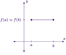
- If the function is constant ,its graph is a horizontal line segment
- In this case, every point satisfies Rolle’s Theorem since the derivative is zero everywhere.
Case 2: The function is not constant
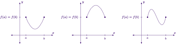
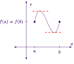
- Since the function is not constant ,it must change directions in order to start and end at same y-value .this means somewhere inside the interval the function will either have a minimum (left hand graph) a maximum (middle graph) or both (right hand graph)
- So, we need to show that at this interior extremum the derivatives must equal zero. The rest of the discussion will focus on the cases where the interior extrema is a maximum, but the discussion for a minimum is largely the same .
- Possibility 1: could the maximum occur at a point where
 ?
? - No, because if
 now the function is increasing. But it can’t increase since we are at its maximum point.
 - Possibility 2: Could the maximum occur at a point where
 ?
? - No, because if
 we know that function is decreasing ,which means it was larger just little to the left of where we are now ,but we are at functions maximum value ,so it could have been larger.
 - Since if
 ,
, but isn’t larger than zero and isn’t smaller than zero,
The only possibility that remains is that 
- And that’s it ! we showed that the function must have an extrema , and that at the extrema the derivative must equal to zero!
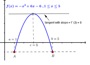
Example:1 Solve the given graph by Rolle’s theorem  is shown below .f(1) =f(5) =-1 and f is continous on
 .
.
Solution: Given  and
and
f(1) =f(5) =-1
Since by Rolle’s theorem, there exists at least one value of x=0 such that 
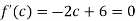
Solve the above equation to obtain
C=3
Therefore at x=3 there is a tangent to the graph of f that has a slope equal to zero(horizontal line ) as shown in figure below.
Example:2 Solve the given graph by Rolle’s theorem  is shown below .f(0)=f(
 =2 and f is continous on
  and differentiable on (0,
Solution: Given  and f(0)=f(
 =2
=2
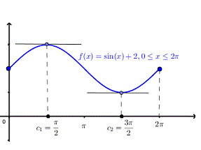
Since by Rolle’s theorem ,there exists at least one value of x=c such that 
The above equation has two solutions on the interval 
Therefore both at x= and x=3
  there are tangents to the graph that have a slope equal to zero (horizontal line ) as shown in figure below.
Example 3: Verify Rolle’s Theorem for the function f(x) = ex(sin x – cos x) in 
Solution: Here f(x) = ex(sin x – cos x); 
i) Ex is an exponential function continuous for every  also sin x and cos x are Trigonometric functions Hence (sin x – cos x) is continuous in
  and Hence ex(sin x – cos x) is continuous in
  .
.
Ii) Consider
f(x) = ex(sin x – cos x)
Diff. w.r.t. x we get
f’(x) = ex(cos x + sin x) + ex(sin x + cos x)
= ex[2sin x]
Clearly f’(x) is exist for each  & f’(x) is not infinite.
Hence f(x) is differentiable in  .
.
Iii) Consider


Also,


Thus 
Hence all the conditions of Rolle’s theorem are satisfied, so there exist  such, that

i.e. 
i.e. sin c = 0


But

Hence Rolle’s theorem is verified.
Lagrange’s Mean Value Theorem:
Statement:
Let f: [a,b] be a continuous function ,differentiable on the open interval (a,b).Thenthere exista some c
 (a,b) such that
f’(c) =
Proof:
We reduce the problem to Rolle’s theorem by using auxillary functions.
Consider,
g(x) = f(x)- 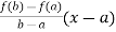
Note: g(a)=g(b)=f(b)
By rolle’s theorem the exists, c in (a,b) such that g’(c) =0 or s
 f’(c) -
  = 0
= 0
Which simplifies to
f’(c) = 
Example 4: Use LaGrange’s mean value theorem to determine a point P on the curve y=
Where the tangent is parallel to the chord joining (2,0) and (3,1)
Solution: Consider y=  in [2,3]
(i) Function is continuous in[2,3] as algebraic expression with positive exponent is continuous.
(ii) y’=  , y’ exists in (2,3) hence the function is derivable in (2,3)
Hence the condition of LMV theorem is satisfied.
Hence, there exists one c in (2,3) such that  =
= 

 =
= 
 4(c-2) = 1
 4c=9
4c=9  c= 4/9
 for x = 9/4, tangent is parallel to the chord joining (2,0) and (3,1)
Substituting in (i) we get,
Y=  =
=  = ½
= ½
Exercise 5: Verify lagrange’s mean value theorem for the following function
f(x) = 
Putting x=a=2 and x=b=5 ,we get
f(2) = 
f(5) = 
Clearly,
f(2)  f(5)
f(5)
Since f(x) is a polynomial function in x, then f(x) is continuous in [2,5].
And f(x) is polynomial in x,then it can be differentiatie such that f’(x) = 4x-7
Then by LMV theorem there exists c  (2,5) such that’
f’ (c) = 
4c-7 = 
 c=3.75
Hence lagrange’s mean value theorem is verified for f(x) in [2,5].
Exercise 6: Verify the Lagrange’s mean value theorem for

Solution: Here f(x) = logx and x
i) Clearly f(x) = log x is logarithmic function. Hence it is continuous in [1, e]
Ii) Consider f(x) = log x.
Diff. w.r.to, x we get,

Clearly f’(x) exists for each value of x & is finite.
Hence all conditions of LMVT are satisfied Hence at least c 
Such that

i.e. 
i.e. 
i.e. 
i.e. 
Since e = 2.7183

Clearly c = 1.7183 
Hence LMVT is verified.
Example 7:Verify mean value theorem for f(x) = tan-1x in [0, 1]
Solution: Here  ;
; 
i) Clearly  is an inverse trigonometric function and hence it is continuous in [0, 1]
Ii) Consider 
Diff. w.r.t. x we get,

Clearly f’(x) is continuous and differentiable in (0, 1) & is finite
Hence all conditions of LMVT are satisfied, Thus there exist 
Such that

i.e. 

i.e. 
i.e. 

i.e. 


Clearly 
Hence LMVT is verified.
Cauchy’s Mean Value Theorem:
Statement:-
If f(x) and g(x) are any two functions such that
a) f(x) and g(x) are continuous in (a, b)
b) both f(x) and g(x) are derivable in (a, b)
c) 
Then for any value of  ,
,  at least
  such that

Exercise 8:Verify Cauchy mean value theorems for  &
& in
in  Solution:Let
  &
& ;
; 
i) Clearly f(x) and g(x) both are trigonometric functions. Hence continuous in 
Ii) Since  &
&
Diff. w.r.t. x we get,
 &
&
Clearly both f’(x) and g’(x) exist & finite in  . Hence f(x) and g(x) is derivable in
  and
and
Iii) 

Hence by Cauchy mean value theorem, there exist at least  such that

i.e. 

i.e. 1 = cot c

i.e. 
Clearly 
Hence Cauchy mean value theorem is verified.
Example 9: Considering the functions ex an e-x, show that c is arithmetic mean of a & b.
Solution: Clearly f(x) and g(x) are exponential functions Hence they are continuous in [a, b].
i) Consider  &
&
Diff. w.r.t. x we get
 and
and 
Clearly f(x) and g(x) are derivable in (a, b)
 By Cauchy’s mean value theorem
  such that

i.e. 
i.e. 
i.e. 
i.e. 
i.e. 
i.e. 

Thus 
i.e. c is arithmetic mean of a & b.
Hence the result
Taylor series:
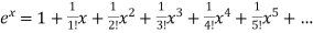
The Taylor’s series can be represented as the following
 (x-a)n
Example 1:
Find the Taylor series for the following:

 =
= 
 <1
<1
 (X/10)<1 and (x/10) > -1
Therefore radius of convergence is (-10,10)
 ROC =10
Example 2:
f(n)5 = 
Here the ROC is 4
Example 2:
Compute the Taylor series centered at zero for f(x)= sinx
Solution:
f(x)=sinx f(0)=0
f’(x) =cosx f’(0)=1
f’’(x)=-sinx f’’(0)=0
f’’’(x) = -cosx f’’’(0)=-1
f(4)(x)= cosx f(4) (0)= 1
Applying Taylor series we get
T(x) =  =
=  = x-
= x-
Thus turns out to converge x to sinx.
Maclaurian series:
Example 3:
 (x)n
(x)n
Example:
f(x)=

= f(0)+f’(0)x+ x2 +
x2 +  x3 +......
= 1+x+x2 +x3 + .....
= 

Example 4:
Find the Maclaurian series for f(x)= ex
Solution:
To get Maclaurian series, we look at the Taylor series polynomials for f near 0 and let them keep going.
Considering for example 

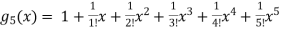
By Maclaurian series we get,
 +
+
By the use of Extended Mean value theorem or cauchy’s mean value theorem ,the L Hospital rule can be proved.
If f and g are two functions on the interval  and differentiable on the interval (a,b) the
 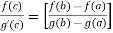 such that c belong to (a,b)
 Assume that the two functions f and g are defined on the interval (c,b) in such away that f(x) 0 and g(x)
 as x
as x
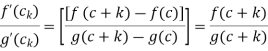
But we have  tends to finite limits .The function f and g are differentiable and
  exists on the set
  , and also f’ and g’ are continuous on the interval
  provided with conditions f(c)=g(c)=0 and g’(c)
By Cauchy mean value theorem states that there exists 
Now , k
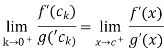
While
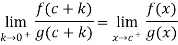
So , we have
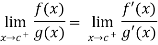
Example:1 :Evaluate
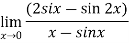
Solution:

Differentiate the above form ,we get
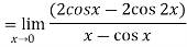
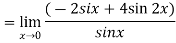
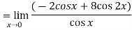
Now substitute the limit,
Therefore ,
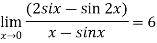
Example 2: Evaluate

Given,


Now substitute the limit

Therefore ,

Example 1:
Find out the maxima and minima of the function
Solution:
Given  …(i)
…(i)
Partially differentiating (i) with respect to x we get
 ….(ii)
Partially differentiating (i) with respect to y we get
 ….(iii)
Now, form the equations 
Using (ii) and (iii) we get


 using above two equations
Squaring both side we get

Or 
This show that 
Also we get 
Thus we get the pair of value as 
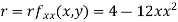
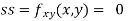
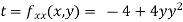
Now, we calculate
Putting above values in
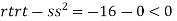
At point (0,0) we get
So, the point (0,0) is a saddle point.
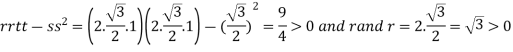
At point  we get

So the point  is the minimum point where
In case 

So the point  is the maximum point where
Example 2:
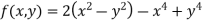
Find the maximum and minimum point of the function
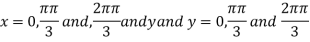
Partially differentiating given equation with respect to and x and y then equate them to zero
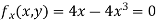
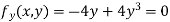
On solving above we get 
Also 
Thus we get the pair of values (0,0), ( ,0) and (0,
Now, we calculate
At the point (0,0)
So function has saddle point at (0,0).
At the point (

So the function has maxima at this point ( .
.
At the point (0,

So the function has minima at this point (0, .
.
At the point (
So the function has an saddle point at (
Example 3:
Find the maximum and minimum value of 
Let 
Partially differentiating given function with respect to x and y and equate it to zero
 ..(i)
..(i)
 ..(ii)
On solving (i) and (ii) we get
Thus pair of values are 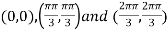
Now, we calculate


At the point (0,0)

So further investigation is required
On the x axis y = 0 , f(x,0)=0
On the line y=x, 
At the point 

So that the given function has maximum value at 
Therefore maximum value of given function
At the point 
So that the given function has minimum value at 
Therefore minimum value of the given function