Unit - 4
Types of Two-Conductor Transmission Lines
The conventional open-wire transmission lines are not suitable for microwave transmission, as the radiation losses would be high. At Microwave frequencies, the transmission lines employed can be broadly classified into three types. They are −
- Co-axial lines
- Strip lines
- Micro strip lines
- Slot lines
- Coplanar lines, etc.
- Rectangular waveguides
- Circular waveguides
- Elliptical waveguides
- Single-ridged waveguides
- Double-ridged waveguides, etc.
- Di-electric rods
- Open waveguides, etc.
Multi-conductor Lines

Fig 1 Cross Sectional view of Co-axial line
Strip Lines
These are the planar transmission lines, used at frequencies from 100MHz to 100GHz.
A Strip line consists of a central thin conducting strip of width ω which is greater than its thickness t. It is placed inside the low loss dielectric (εr) substrate of thickness b/2 between two wide ground plates. The width of the ground plates is five times greater than the spacing between the plates.
The thickness of metallic central conductor and the thickness of metallic ground planes are the same. The following figure shows the cross-sectional view of the strip line structure.
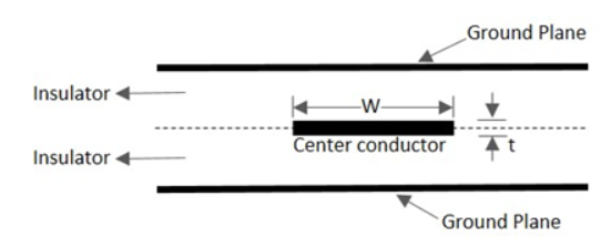
Fig 2 Strip Line Transmission Line
Micro Strip Lines
The strip line has a disadvantage that it is not accessible for adjustment and tuning. This is avoided in micro strip lines, which allows mounting of active or passive devices, and also allows making minor adjustments after the circuit has been fabricated.
A micro strip line is an unsymmetrical parallel plate transmission line, having di-electric substrate which has a metallized ground on the bottom and a thin conducting strip on top with thickness 't' and width 'ω'. This can be understood by taking a look at the following figure, which shows a micro strip line.
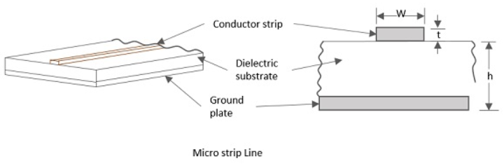
Fig 3 Micro Strip Line
The characteristic impedance of a micro strip is a function of the strip line width ω, thickness t and the distance between the line and the ground plane h. Micro strip lines are of many types such as embedded micro strip, inverted micro strip, suspended micro strip and slotted micro strip transmission lines.
In addition to these, some other TEM lines such as parallel strip lines and coplanar strip lines also have been used for microwave integrated circuits.
Key takeaway
The cost of micro strip is very high as compared to co-axial and two wire line. The micro strip line cannot be used as a transmission line when the distance between source and load is long. This type of transmission line cannot be used in twisty paths between source and load.
A transmission line is a means of transfer of information from one point to another. Usually, it consists of two conductors. It is used to connect a source to a load. The source may be a transmitter and the load may be a receiver.
The performance of transmission line depends on the parameters of the line. The transmission line has mainly four parameters, resistance, inductance, capacitance and shunt conductance. These parameters are uniformly distributed along the line. Hence, it is also called the distributed parameter of the transmission line.
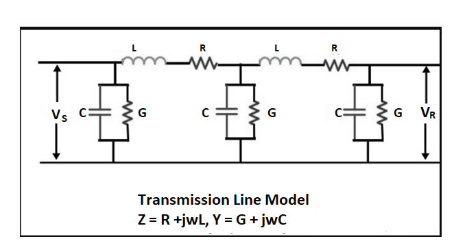
Fig 4 Transmission Line
The various notations used in this derivation are,
 Series resistance, ohms per unit length, including both the wires
 Series inductance, henry per unit length
 Capacitance between the conductors, farads per unit length
G = shunt leakage conductance between the conductors, mhos per unit length
ωL = Series reactance in per unit length
ωC= Shunt susceptance in mhos per unit length
S=R+jωL=Series impedance in ohms per unit length
Y=G+ωC=Shunt admittance in mhos per unit length
s = Distance up to point of consideration, measured from receiving end
J = Current in the line at any point
E = Voltage between the conductors at any point
 = Length of the line
The transmission line of length l can be considered to be made up of infinitesimal T sections. One such section of length ds is shown in figure. It carries current I.
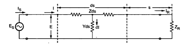
Fig 5 Circuit Diagram of Transmission Line
The point under consideration is at a distance s from the receiving end. The length of section is ds hence its series impedance is Zds and shunt admittance is Yds. The current is I and voltage E.
The elemental voltage drop in the length ds is

 (1)
(1)
The leakage current flowing through shunt admittance from one conductor to other is given by,
 (2)
(2)

Differentiating equations (1) and (2) with respect to s we get


and This is because both E and I are functions of s.
 (3)
(3)
 (4)
(4)
The equations (3) and (4) are the second order differential equations describing the transmission line having distributed constants all along its length. It is necessary to solve these equations to obtain expressions of E and I.
Replace the operator d/ds by m we get

 (5)
(5)
So there exists two solutions for positive sign of m and negative side of m. The general solution for E and I are
 (6)
(6)
 (7)
(7)
Where A, B, C and D are arbitrary constants of integration
To obtain A, B, C, D
As distance is measured from receiving end  indicates the receiving end.
 and
and  at
at 
Substitute in the solution
 …. (8(a))
 …. 8(b)
Same condition can be used in the equations obtained by differentiating the equations (6) and (7) with respect to s.

and 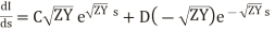
But  and
and 
 (9)
(9)
And  (10)
(10)

 (11)
(11)
And  (12)
(12)
Now use 
 (13(a))
 (13(b))
The equations 8a, 8b13a and 14b are to be solved simultaneously to obtain the values of the constants A, B, C and D.
Now while solving these equations use the results,

Taking LCM as  and taking
  out from equation (18)
 … (20)
Taking LCM as  and taking
  out from equation (19)
 … (21)
The negative sign is used to convert 
The equations (20) and (21) is the genral solution of a transmission line
Another way of representing the equation is,


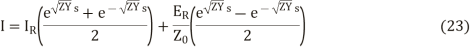
But 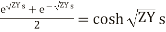 and
and 
 (24)
(24)
And  (25)
(25)
The equation (24) and (25) give the values of E and I at any point along the length of the line.
If x is the distance measured down the line from the sending end
And the equation (24) and (25) get transferred interms of  and
and  as,
as,
 (26)
(26)
 (27)
(27)
And  as derived earlier and hence equations can be written interms of propogation constant .
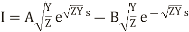
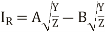
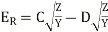
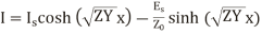
Summarizing,
If receiving end parameters are known and s is distance measured from the receiving end then,

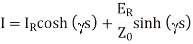
And if sending end parameters are known and x is distance measured from the sending end then,


An ideal transmission line has these properties:
Sufficient conditions for building an ideal transmission line are that you have two perfect conductors with zero resistance, uniform cross section, separation much smaller than the wavelength of the signals conveyed, and a perfect (lossless) dielectric. Voltages impressed upon one end of such an ideal transmission line will propagate forever, at constant velocity, without distortion or attenuation.
The propagation velocity, or transmission velocity, of a line is rated in units of m/s. The symbol for propagation velocity is v. This quantity indicates how far your signals will travel in every unit of time. For the case of perfect, zero-resistance conductors surrounded by a perfect vacuum, the propagation velocity equals c, the velocity of light in a vacuum, approximately 2.998 ·10 8 m/s.
The characteristic impedance of an ideal transmission line remains constant at all frequencies. It has no imaginary part and is not a function of frequency. It is a function only of the physical geometry of the transmission line and the dielectric constant of the insulation.
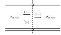
Fig 6 Transmission-line junction for illustrating reflection and transmission resulting from an incident wave
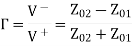
Find that the wave alone cannot satisfy the boundary condition at the junction, since the voltage-to-current ratio for that wave is whereas the characteristic impedance of line 2 is Hence, a reflected wave and a transmitted wave are set up such that the boundary conditions are satisfied. Let the voltages and currents in these waves be and respectively, where the superscript denotes that the transmitted wave is a wave resulting from the incident wave. We then have the situation shown in Figure below.

Fig 6 (a) For obtaining the reflected wave and transmitted wave voltages and currents for the system of Fig 6 (b) Equivalent to (a) for using the reflection coefficient concept.
Using the boundary conditions at the junction, we then write

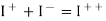
But we know that and H

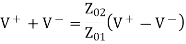
Thus, to the incident wave, the transmission line to the right looks like its characteristic impedance as shown in Figure (b). The difference between a resistive load of and a line of characteristic impedance is that, in the first case, power is dissipated in the load, whereas in the second ease, the power is transmitted into the line
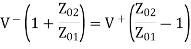
We now define the voltage transmission coefficient, denoted by the symbol as the ratio of the transmitted wave voltage to the incident wave voltage. Thus,

The current transmission coefficient, which is the ratio of the transmitted wave current to the incident wave current, is given by
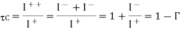
At this point, one may be puzzled to note that the transmitted voltage can be greater than the incident voltage if is positive. However, this is not of concern, since then the transmitted current will be less than the incident current. Similarly, the transmitted current is greater than the incident current when is negative, but then the transmitted voltage is less than the incident voltage. In fact, what is important is that the transmitted power is always less than (or equal to) the incident power since


Key takeaway:
The voltage transmission coefficient, denoted by the symbol as the ratio of the transmitted wave voltage to the incident wave voltage. Thus,
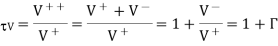

Figure 8. Mismatch
The solution for this is to place a matching network between the line and the load.

Figure 9. Matching network
The quarter-wave transformer is simply a transmission line with characteristic impedance Z1 and length l = λ/4 (i.e., a quarter-wave line).

Figure 10. λ/4 matching network
We know that the input impedance of the quarter wavelength line is:
Zin = (Z1) 2/ ZL = (Z1) 2/ RL
Thus, if we wish for Zin to be numerically equal to Z0, we find:
Zin = (Z1) 2/ RL = Zo
Solving for Z1, we find its required value to be:
Z1 = √Zo RL
Therefore, a λ/4 line with characteristic impedance 𝑍1 =  𝑍0𝑅𝐿 will match a transmission line with characteristic impedance Z0 to a resistive load RL

Figure 11. Power delivered to load.
Single-Stub Matching Technique
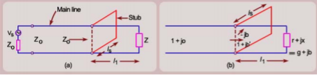
Fig 12 Single Stub Matching Technique
Since we have a parallel connection of transmission lines, it is more convenient to solve the problem using admittances rather than impedances. To convert the impedance into admittance also we make use of the Smith chart and avoid any analytical calculation. Now onwards treat the Smith chart as the admittance chart

Matching Procedure
First mark the load admittance on the admittance smith chart (A). Plot the constant  circle on the smith chart. Move on the constant
  circle till you intersect the constant g=1 circle this point of intersection corresponds to point 1+jb’ (B). The distance traversed on the constant circle is l1. This is the location of placing the stub on the transmission line from the load end. Find constant susceptance jb’ circle. Find mirror image of the circle to get -jb’ circle. Mark 0-jb’ on the outer most circle (D). From (D) move circular clockwise up to s.c point (E) to get the stub length ls.
Key Takeaway:
A quarter-wave transformer is a simple impedance transformer which is commonly used in impedance matching in order to minimize the energy which is reflected when a transmission line is connected to a load.
References:


