Unit - 5
Analog Filters
The Impulse Invariance Method is used to design a discrete filter that yields a similar frequency response to that of an analog filter. Discrete filters are amazing for two very significant reasons:
We can design this filter by finding out one very important piece of information i.e., the impulse response of the analog filter. By sampling the response we will get the time-domain impulse response of the discrete filter.
When observing the impulse responses of the continuous and discrete responses, it is hard to miss that they correspond with each other. The analog filter can be represented by a transfer function, Hc(s).
Zeros are the roots of the numerator and poles are the roots of the denominator.
Mapping from s-plane to z-plane
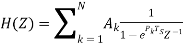
The transfer function of the analog filter in terms of partial fraction expansion with real coefficients is
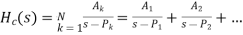 Where A are the real coefficients and P are the poles of the function And k can be 1, 2 …N.
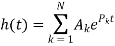
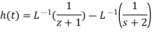
h(t) is the impulse response of the same analog filter but in the time domain. Since ‘s’ represents a Laplace function Hc(s) can be converted to h(t), by taking its inverse Laplace transform.
Using this transformation,
We obtain
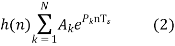
However, in order to obtain a discrete frequency response, we need to sample this equation. Replace ‘nTS’ in the place of t where TS represents the sampling time. This gives us the sampled response h(n),
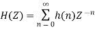
Now, to obtain the transfer function of the IIR Digital Filter which is of the ‘z’ operator, we have to perform z-transform with the newly found sampled impulse response, h(n). For a causal system which depends on past(-n) and current inputs (n), we can get H(z) with the formula shown below
We have already obtained the equation for h(n). Hence, substitute eqn (2) into the above equation
Factoring the coefficient and the common power of n —(3)
Based on the standard summation formula, (3) is modified and written as the required transfer function of the IIR filter.
 –(4)
–(4)
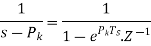
Hence (4) is obtained from (1), by mapping the poles of the analog filter to that of the digital filter.
That is how you map from the s-plane to z-plane
Relationship of S-plane to Z plane
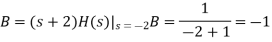
From the equation above, Since, the poles are the denominators we can say  .
.
Comparing (1) and (4), we can derive that
 –(5)
–(5)
and since  , substituting into (5) gives us
 –(6)
–(6)
where
TS is the sampling time
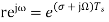
Now, s is taken to be the Laplace operator
 –(7)
–(7)
σ is the attenuation factor
Ω is the analog frequency
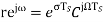
Changing Z from rectangular coordinates to the polar coordinates, we get:
 –(8)
–(8)
where r is magnitude and ω is digital frequency
Replacing (7) in place of s in (6), and replacing that value as Z in (8)
Compare the real and imaginary parts separately. Where the component with ‘j’ is imaginary.
 –(9)
–(9)
and

Hence, we can make the inference that

To understand the relationship between the s-plane and Z-plane, we need to picture how they will be plotted on a graph. If we were to plot (7) in the ‘s’ domain, σ would be the X-coordinates and jΩ would be the Y-coordinate. Now, if we were to plot (8) in the ‘Z’ domain, the real portion would be the X-coordinate, and the imaginary part would be the Y-coordinate.
Let us take a closer look at equation (9),

There are a few conditions that could help us identify where it is going to be mapped on the s-plane.
Case 1
when σ <0, it would translate that r is the reciprocal of ‘e’ raised to a constant. This will limit the range of r from 0 to 1.
Since σ <0, it would be a negative value and would be mapped on the left-hand side of the graph in the ‘s’ domain
Since 0<r<1, this would fall within the unit circle which has a radius of in the ‘z’ domain.
Case 2
When σ =0, this would make r=e0, which gives us 1, which means r=1. When the radius is 1, it is a unit circle.
Since σ =0, which indicates the Y-axis of the ‘s’ domain.
Since r=1, the point would be on the unit circle in the ‘z’ domain.
Case 3
When σ>0, since it is positive, r would be equal to ‘e’ raised to a particular constant, which means r would also be a positive value greater than 1.
Since σ>0, the positive value would be mapped onto the right-hand side of the ‘s’ domain.
Since r>1, the point would be mapped outside the unit circle in the ‘z’ domain.
Here is a pictorial representation of the three cases:
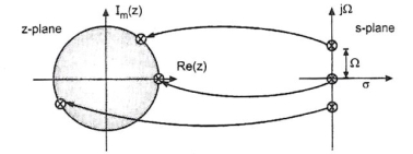
Mapping of poles located at the imaginary axis of the s-plane onto the unit circle of the z-plane. This is an important condition for accurate transformation.
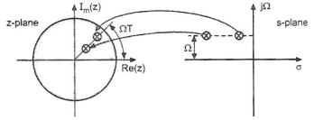
Mapping of the stable poles on the left-hand side of the imaginary s-plane axis into the unit circle on the z-plane. Poles on the right-hand side of the imaginary axis of the s-plane lie outside the unit circle of the z-plane when mapped.
Disadvantages:
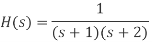
Given 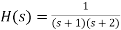 , that has a sampling frequency of 5Hz. Find the transfer function of the IIR digital filter.
Solution:
Step 1:
Step 2:
Applying partial fractions on H(s),

Step 3:
Step 4:
 )
)
Key takeaway
when σ <0, it would translate that r is the reciprocal of ‘e’ raised to a constant. This will limit the range of r from 0 to 1.
When σ =0, this would make r=e0, which gives us 1, which means r=1. When the radius is 1, it is a unit circle.
When σ>0, since it is positive, r would be equal to ‘e’ raised to a particular constant, which means r would also be a positive value greater than 1.
Poles on the right-hand side of the imaginary axis of the s-plane lie outside the unit circle of the z-plane when mapped.
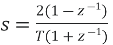
The bilinear transform is the result of a numerical integration of the analog transfer function into the digital domain. We can define the bilinear transform as:
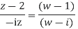
Find the bilinear transformation which maps points z =2,1,0 onto the points w=1,0,i.
Ans. Let, 
And, 
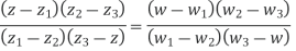
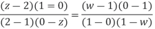
Since bilinear transformation preserves cross ratios,
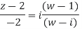
Thus we have,
Use the bilinear transformation to convert the analog filtrt with system function
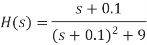
 into a digital IIR filter. Select T =0.1
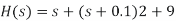
Consider the following system function

Note that the following is the resonant frequency of the analog filter

Consider that the resonant frequency of analog filter must be mapped by selecting the value of parameter
T= 0,1
Use the following mapping for bilinear transformation
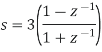
Write the system function H(z) of the resultant digital filter
Frequency warping
• The bilinear transformation method has the following important features: A stable analog filter gives a stable digital filter. t The maxima and minima of the amplitude response in the analog filter are preserved in the digital filter. As a consequence, – the pass band ripple, and – the minimum stop band attenuation of the analog filter are preserved in the digital filter frame.
• To determine the frequency response of a continuous-time filter, the transfer function Ha(s)Ha(s) is evaluated at s=jω which is on the jω axis. Likewise, to determine the frequency response of a discrete-time filter, the transfer function Hd(z) is evaluated at z=ejωT which is on the unit circle, |z|=1|z|=1 .
• When the actual frequency of ω is input to the discrete-time filter designed by use of the bilinear transform, it is desired to know at what frequency, ωa , for the continuous-time filter that this ω is mapped to.
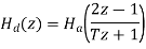
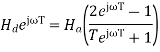
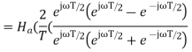
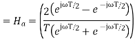
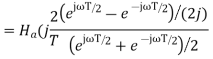
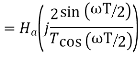
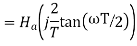
• This shows that every point on the unit circle in the discrete-time filter z-plane, z= ejωT is mapped to a point on the jω axis on the continuous-time filter s-plane, s=jω. That is, the discrete-time to continuous-time frequency mapping of the bilinear transform is
ωa=(2/T) tan(ωt/2)
and the inverse mapping is
ω=(2/T) arc tan(ωaT/2)
• The discrete-time filter behaves at frequency the same way that the continuous-time filter behaves at frequency (2/T)tan(ωT/2). Specifically, the gain and phase shift that the discrete-time filter has at frequency ω is the same gain and phase shift that the continuous-time filter has at frequency (2/T)tan(ωT/2). This means that every feature, every "bump" that is visible in the frequency response of the continuous-time filter is also visible in the discrete-time filter, but at a different frequency. For low frequencies (that is, when ω≪2/T or ωa≪2/T),ω≈ωa.
One can see that the entire continuous frequency range
−∞<ωa<+∞
is mapped onto the fundamental frequency interval
−πT<ω<+πTω=±π/T.ωa=±∞
One can also see that there is a nonlinear relationship between ωa and ω This effect of the bilinear transform is called frequency warping.

Fig 1 Frequency wrapping
Design a discrete time lowpass filter to satisfy the following amplitude specifications: 
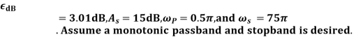
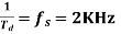
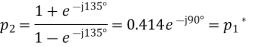
The pre-warped critical frequency are
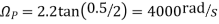
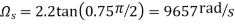

Since both the passband and stopband are required to be monotonic, a Butterworth approximation will be used
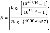

From the Butterworth design tables we can immediately write
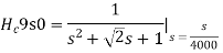
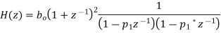
Now find H (z) by first noting that 

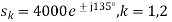
Using the pole/ zero mapping formula
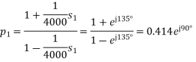
We can now write
Find  by setting
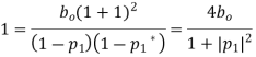
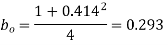
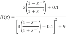
Finally after multiplying out the numerator and denominator we obtain
Key takeaway
Sr No. | Impulse Invariance | Bilinear Transformation |
1 | In this method IIR filters are designed having a unit sample response h (n) that is sampled version of the impulse response of the analog filter. | This method of IIR filter design is based on the trapezoidal formula for numerical integration. |
2 | The bilinear transformation is a conformal mapping that transforms the j | The bilinear transformation is a conformal mapping tjat transforms the |
3 | For design of LPF, HPF and almost all types of bandpass and band stop filters this method is used. | For designing of LPF, HPF and almost all types of bandpass and band stop filters this method is used. |
4 | Frequency relationship is non –linear. Frequency warping or frequency compression is due to non – linearity. | Frequency relationship is non linear. Frequency warping or frequency compression is due to non – linearity. |
5 | All poles are mapped from s plane to the z plane by the relationship | All poles and zeros are mapped. |


Since adaptive FIR filters have only adjustable zeros, they are free of stability problems that can be associated with adaptive IIR filters where both poles and zeros are adjustable. Of the various FIR filter structures available, the direct form (transversal), the symmetric transversal form, and the lattice form are the ones often employed in adaptive filtering applications.
Adaptive filters are widely used in telecommunications, control systems, radar systems, and in other systems where minimal information is available about the incoming signal. Due to the variety of implementation options for adaptive filters, many aspects of adaptive filter design, as well as the development of some of the adaptive algorithms, are governed by the applications themselves. Several applications of adaptive filters based on FIR filter structures are described below.
Transversal Structure
w(n) = [w0(n) w1(n) ... wN-1(n)] T
The tap-input vector, u(n), as
u(n) = [u(n) u(n-1) ... u(n-N+1)] T
The FIR filter output, y(n), can then be expressed as
y(n) = wT(n) u(n) = 
Where T denotes transpose, n is the time index and N is the order of the filter.
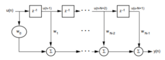
Fig 2 Transversal FIR Filter Structure
Symmetric Transversal Structure
w0(n) = wN – 1(n), w1(n) = wN - 2(n)... has a linear phase response in the frequency domain.
Consequently, the number of weights is reduced by a half in a transversal structure, as shown in Figure below with an even N tap weight. The tap-input vector becomes
u(n) = [u(n) + u(n – N +1 ), u(n – 1) + u(n – N + 2), ... ,u(n – N/2 + 1) + u(n - N/2)] T
As a result, the filter output y(n) becomes
y(n) = 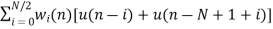
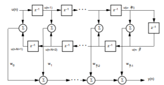
Fig 3 Symmetric Transversal Filter Structure
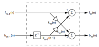
Lattice Structure
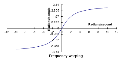
Fig 4 Lattice Structure
The lattice structure offers several advantages over the transversal structure:
• The lattice structure has good numerical round-off characteristics that make it less sensitive than the transversal structure to round-off errors and parameter variations.
• The lattice structure orthogonalizes the input signal stage-by-stage, which leads to fast convergence and efficient tracking capabilities when used in an adaptive environment.
• The various stages are decoupled from each other, so it is relatively easy to increase the prediction order if required.
• The lattice filter (predictor) can be interpreted as wave propagation in a stratified medium. This can represent an acoustical tube model of the human vocal tract, which is extremely useful in digital speech processing. These advantages, however, come at the expense of an increased number of multiplies and adds for a given transfer function realization.
The following equations represent the dynamics of the mth stage of an order M lattice structure as derived from Figure above:
fm(n)=fm – 1(n) – Km(n) bm – 1(n – 1), 0 < M
bm(n)=bm – 1(n – 1) Km(n) fm – 1(n), 0 < m < M
where fm(n) represents the forward prediction error, bm(n) represents the backward prediction error, Km(n) is the reflection coefficient, m is the stage index, and M is the number of cascaded stages. Km(n) has a magnitude less than one.
The terms fm(n) and bm(n) are initialized as f0(n) = b0(n) = u(n) where u(n) is the input signal. Speech analysis is usually performed by using the lattice structure and the reflection coefficients Km(n). Since the dynamic range of Km(n) is significantly smaller than that of the tap weights, w(n), of a transversal filter, the reflection coefficients require fewer bits to represent them. Hence, Km(n) are transmitted over the channel.
Adaptive Filter Algorithms
Two types of adaptive algorithms are discussed in this section: least-mean square (LMS) and recursive least-squares (RLS). LMS algorithms are based on a gradient-type search for tracking time-varying signal characteristics. RLS algorithms provide faster convergence and better tracking of time variant signal statistics than LMS algorithms, but are more complex computationally.
w(n+1) = w(n) + µe(n)u(n)
where w(n) represents the tap weights of the transversal filter, e(n) is the error signal, u(n) represents the tap inputs, and the factor µ is the adaptation parameter or step-size. To ensure convergence, µ must satisfy the condition
0 < µ < (2 / total input power)
where the total input power refers to the sum of the mean-square values of the tap inputs u(n), u(n-1), ..., u(n-N+1). Moreover, the LMS convergence time depends on the ratio of maximum to minimum eigenvalues of the autocorrelation matrix R of the input signal. To insure, that µ does not become sufficiently large to cause filter instability, a Normalized LMS algorithm can be employed. The normalized LMS employs a time-varying mu defined as
mu=x/uT(n).u(n)
where x is the normalized step-size chosen between 0 and 2. Tap weights are updated according to the relationship
w(n+1) = w(n) +xe(n)u(n)/[r+uT(n)u(n)]
The term x is the new normalized adaptation constant, while r is a small positive term included to ensure that the update term does not become excessively large when uT(n)u(n) temporarily becomes small. A problem can occur when the autocorrelation matrix associated with the input process has one or more zero eigenvalues. In this case, the adaptive filter will not converge to a unique solution. In addition, some uncoupled coefficients (weights) may grow without bound until hardware overflow or underflow occurs. This problem can be remedied by using coefficient leakage. This “leaky” LMS algorithm can be written as
w(n+1) = (1-µr )w(n) + µe(n)u(n)
where the adaptation constant µ and the leakage coefficient r are a small-positive values.
The RLS Algorithm
For faster rates of convergence, more complex algorithms with additional parameters must be used. The RLS algorithm uses a least-squares method to estimate correlation directly from the input data. The LMS algorithm uses the statistical mean-squared-error method, which is slower. The RLS algorithm uses a transversal FIR filter implementation. The order of operations the algorithm takes is
1. Compute the filter output (tap weights initialized to zero)
2. Find the error signal
3. Compute the Kalman Gain Vector (defined below)
4. Update the inverse of the correlation matrix
5. Update the tap weights
The Kalman Gain Vector is based on input-data autocorrelation results, the input data itself, and a factor called the forgetting factor. The forgetting factor ranges between zero and one and provides a time-weighting of the input data such that the most recent data points are weighted more heavily than past data. This allows the filter coefficients to adapt to time varying statistical characteristics of the input data. The tap weight update is based on the error signal and the Kalman Gain Vector and is expressed as
w(n) = w(n-1) + Ke(n)
where K is the Kalman Gain Vector and e(n) represents the error signal.
Key takeaway
Parameter | Adaptive filtering algorithm | ||
Least Mean Square (LMS) | Normalized LMS (NLMS) | Recursive Least Square (RLS) | |
Convergence | Very Slow | Convergence | Very Slow |
Stability | Very Stable | Stability | Very Stable |
Complexity | Very Low | Complexity | Very Low |
Consumption | Very Low | Consumption | Very Low |
Implementation | Very Simple | Implementation | Very Simple |
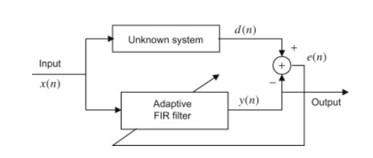
Another application of the adaptive filter is system modeling. The adaptive filter can keep tracking the behaviour of an unknown system by using the unknown system input and output.
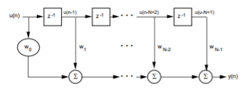
Fig5 System Modeling
As shown in the figure, after the adaptive filter converges, the adaptive filter output y(n) will be as close as possible to the unknown system's output. Since both the unknown system and the adaptive filter respond the same input, the transfer function of the adaptive filter will approximate that of the unknown system.
Inverse Modeling
The inverse modeling is an application that can be used in the area of channel equalization, for example it is applied in modems to reduce channel distortion resulting from the high speed of data transmission over telephone channels. In order to compensate the channel distortion, we need to use an equalizer, which is the inverse of the channel’s transfer function.
High-speed data transmission through channels with severe distortion can be achieved in several ways, one way is to design the transmit and receive filters so that the combination of filters and channel results in an acceptable error from the combination of inter symbol interference and noise; and the other way is designing an equalizer in the receiver that counteracts the channel distortion. The second method is the most commonly used technology for data transmission applications.
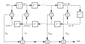
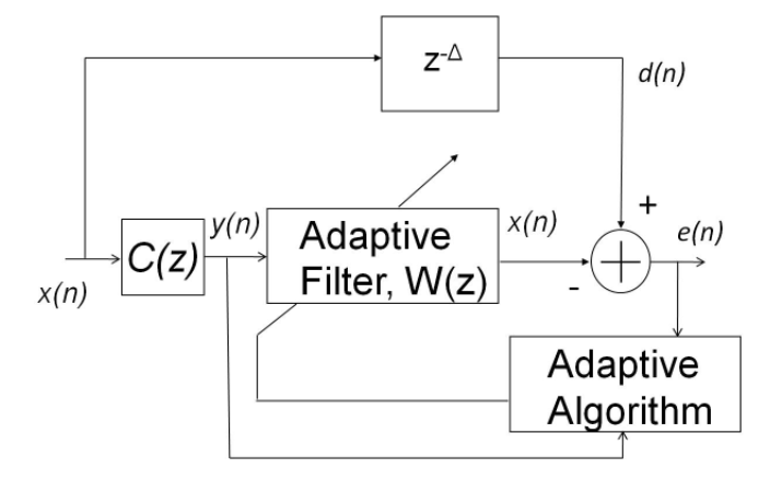
Fig6 Inverse Modeling
Figure shows an adaptive channel equalizer, the received signal y(n) is different from the original signal x(n) because it was distorted by the overall channel transfer function C(z), which includes the transmit filter, the transmission medium, and the receive filter.
To recover the original signal x(n), y(n) must be processed using the equalizer W(z), which is the inverse of the channel’s transfer function C(z) in order to compensate for the channel distortion. Therefore, the equalizer must be designed by
W(z)=1/C(z)
In practice, the telephone channel is time varying and is unknown in the design stage due to variations in the transmission medium. Thus, it is needed an adaptive equalizer that provides precise compensation over the time-varying channel. The adaptive filter requires the desired signal d(n) for computing the error signal e(n) for the LMS algorithm. An adaptive filter requires the desired signal d(n) for computing the error signal e(n) for the LMS algorithm.
The delayed version of the transmitted signal x(n - Δ) is the desired response for the adaptive equalizer W(z). Since the adaptive filter is located in the receiver, the desired signal generated by the transmitter is not available at the receiver. The desired signal may be generated locally in the receiver using two methods. During the training stage, the adaptive equalizer coefficients are adjusted by transmitting a short training sequence. This known transmitted sequence is also generated in the receiver and is used as the desired signal d(n) for the LMS algorithm.
After the short training period, the transmitter begins to transmit the data sequence. In the data mode, the output of the equalizer x(n) is used by a decision device to produce binary data. Assuming that the output of the decision device is correct, the binary sequence can be used as the desired signal d(n) to generate the error signal for the LMS algorithm.
Key takeaway
In inverse modelling to recover the original signal x(n), y(n) must be processed using the equalizer W(z), which is the inverse of the channel’s transfer function C(z) in order to compensate for the channel distortion.
DFT
Enter the sequence x= [4 5 6 9]
Enter the length of the DFT N= 7
Columns 1 through 4
24.0000 -2.3264 -13.6637i 3.0930 + 4.7651i
1.2334 - 6.2528i
Columns 5 through 7
1.2334 + 6.2528i 3.0930 - 4.7651i -2.3264 +13.6637i
Output
FFT
% for defined sequence using inbuilt function
n = 0:6;
x = [4 6 2 1 7 4 8];
a = fft(x);
mag = abs(a);
pha = angle(a);
subplot(2,1,1);
plot(mag);
grid on
title('Magnitude Response');
subplot(2,1,2);
plot(pha);
grid on
title('phase Response');
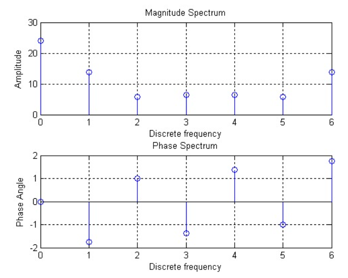
2) Implementation of FFT of given sequence in matlab n-point fft WITHOUT USING INBUILT FUNCTION
Code
close all;
clc;
x=input('Enter the sequence x[n]= ');
N=input('Enter the value N point= ');
L=length(x);
x_n=[x,zeros(1,N-L)];
for i=1:N
for j=1:N
temp=-2*pi*(i-1)*(j-1)/N;
DFT_mat(i,j)=exp(complex(0,temp));
end
end
X_k=DFT_mat*x_n';
disp('N point DFT is X[k] = ');
disp(X_k);
mag=abs(X_k);
phase=angle(X_k)*180/pi;
subplot(2,1,1);
stem(mag);
xlabel('frequency index k');
ylabel('Magnitude of X[k]');
axis([0 N+1 -2 max(mag)+2]);
subplot(2,1,2);
stem(phase);
xlabel('frequency index k');
ylabel('Phase of X[k]');
axis([0 N+1 -180 180]);
PROGRAM: for user defined sequence
clc;
clear all;
close all;
tic;
x=input('enter the sequence');
n=input('enter the length of fft'); %compute fft
disp('fourier transformed signal');
X=fft(x,n)
subplot(1,2,1);stem(x); title('i/p signal');
xlabel('n --->');
ylabel('x(n) -->');grid;
subplot(1,2,2);stem(X);
title('fft of i/p x(n) is:');
xlabel('Real axis --->');
ylabel('Imaginary axis -->');grid;
OUTPUT
enter the sequence[1 .25 .3 4]
enter the length of fft4
fourier transformed signal
X =
5.5500 0.7000 + 3.7500i -2.9500 0.7000 - 3.7500i
Graph output
Z-transform
close all;
syms n;
a=2;
x=a^n;
X=ztrans(x); %finding z transform
disp('z transform of a^n a>1');
disp(X);
syms n;
a=0.5;
x=a^n;
X1=ztrans(x);
disp('z transform of a^n 0<a<1');
disp(X1);
syms n;
a=2;
x=1+n;
X2=ztrans(x);
disp('z transform of 1+n');
disp(X2);
A=iztrans(X);
disp('inverse z transform of a^n a>1');
disp(A);
B=iztrans(X1);
disp('inverse z transform of a^n 0<a<1');
disp(B);
C=iztrans(X2);
disp('inverse z transform of 1+n');
disp(C);
subplot(1,3,1);
zplane([1 0],[1 -2]);
subplot(1,3,2);
zplane([1 0],[1 -1/2]);
subplot(1,3,3);
zplane([1 0 0],[1 -2 1]);
OUTPUT:
z transform of a^n 0<a<1
z/(z - 1/2)
z transform of 1+n
z/(z - 1) + z/(z - 1)^2
inverse z transform of a^n a>1
2^n
inverse z transform of a^n 0<a<1
(1/2)^n
inverse z transform of 1+n
n + 1
H(s) = (s+2)/(s2+3s+2)
Code
num=[1 2];
den= [1 3 2];
sys=tf(num,den)
sys2=c2d(sys,0.1)
step(sys)
hold on step(sys2)
Output
For continuous system (s+2)/(s2+3s+2)
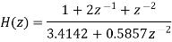
For discrete time system (0.095z-0.077)/(z2-1.724z+0.7408)
syms z k
F=z/(z-0.5);
a=iztrans(F,k)
pretty(a)
Output
a= (0.5) k
IIR Adaptive Filter
% LMS used in a simple system identification application.
% By the end of this script the adaptive filter w should
% have the same coefficients as the unknown filter h.
% iter = 5000; % Number of samples to process
% Complex unknown impulse response
h = [.9 + i*.4; 0.7+ i*.2; .5; .3+i*.1; .1];
xn = 2*(rand(iter,1)-0.5);
% Input signal, zero mean random.
% although xn is real, dn will be complex since h is complex
dn = osfilter(h,xn); % Unknown filter output
en = zeros(iter,1); % vector to collect the error
% Initialize the LMS algorithm with a filter of 10 coef. [w,x,d,y,e]=init_lms(10);
%% Processing Loop
for (m=1:iter)
x = [xn(m); x(1:end-1)]; % update the input delay line
d = dn(m,:) + 1e-3*rand; % additive noise of var = 1e-6
% call LMS to calculate the output, estimation error
% and update the coefficients.
[w,y,e]= asptlms(x,w,d,0.05);
% save the last error sample to plot later
en(m) = e;
end;
% display the results
% note that w converges to conj(h) for complex data
subplot(2,2,1);stem([real(w) imag(conj(w))]); grid;
subplot(2,2,2);eb = filter(.1,[1 -.9], en .* conj(en));
plot(10*log10(eb ));grid
Output
FIR Adaptive Filter
Adaptive Noise Cancellation using Least Mean Square Filter Algorithm
clc; |
close all; |
clear all; |
order=3; |
NN=10000; |
[y1,Fs]=wavread('a1'); |
y = (y1(1:NN))'; |
time=(1/22050)*200; |
N=length(y); |
xlabel('time (sec)'); |
ylabel('relative signal strength') |
subplot(5,1,1); plot(y); |
n1 = randn(1,NN); |
n1 = n1/max(abs(n1)); |
subplot(5,1,2); plot(n1); |
x = y + 0.1*n1; |
subplot(5,1,3); plot(x); |
subplot(5,1,4) |
plot(ref) |
title('reference (noisy noise) (input2)'); |
wall = []; |
w=0.1*zeros(order,1); |
mu=0.04; |
for i=1:N-order |
buffer = ref(i:i+order-1); %current 32 points of reference |
desired(i) = x(i)-buffer*w; %dot product reference and coeffs |
w=w+(buffer.*mu*desired(i)/norm(buffer))'; %update coeffs |
wall = [wall,w]; |
end |
subplot(5,1,5) |
plot(desired) |
title('Adaptive output (hopefully it''s close to "voice")') |
color = ['b','r','m','k','g','c','y','b','r','m','k','g','c','y']; |
figure; |
for pp = 1 : order |
plot(wall(pp,:),color(pp)); |
hold on; |
end |
clc; |
close all; |
clear all; |
order=3; |
NN=10000; |
[y1,Fs]=wavread('a1'); |
y = (y1(1:NN))'; |
time=(1/22050)*200; |
N=length(y); |
xlabel('time (sec)'); |
ylabel('relative signal strength') |
subplot(5,1,1); plot(y); |
n1 = randn(1,NN); |
n1 = n1/max(abs(n1)); |
subplot(5,1,2); plot(n1); |
x = y + 0.1*n1; |
subplot(5,1,3); plot(x); |
ref=x+.1*rand; %noisy noise |
subplot(5,1,4) |
plot(ref) |
title('reference (noisy noise) (input2)'); |
wall = []; |
w=0.1*zeros(order,1); |
mu=0.04; |
for i=1:N-order |
buffer = ref(i:i+order-1); %current 32 points of reference |
desired(i) = x(i)-buffer*w; %dot product reference and coeffs |
w=w+(buffer.*mu*desired(i)/norm(buffer))'; %update coeffs |
wall = [wall,w]; |
end |
subplot(5,1,5) |
plot(desired) |
title('Adaptive output (hopefully it''s close to "voice")') |
color = ['b','r','m','k','g','c','y','b','r','m','k','g','c','y']; |
figure; |
for pp = 1 : order |
plot(wall(pp,:),color(pp)); |
hold on; |
end |
References:
1. S. K. Mitra, “Digital Signal Processing: A computer based approach”, McGraw Hill, 2011.
2. A.V. Oppenheim and R. W. Schafer, “Discrete Time Signal Processing”, Prentice Hall, 1989.
3. J. G. Proakis and D.G. Manolakis, “Digital Signal Processing: Principles, Algorithms And Applications”, Prentice Hall, 1997.
4. L. R. Rabiner and B. Gold, “Theory and Application of Digital Signal Processing”, Prentice Hall, 1992.
5. J. R. Johnson, “Introduction to Digital Signal Processing”, Prentice Hall, 1992.
6. D. J. DeFatta, J. G. Lucas andW. S. Hodgkiss, “Digital Signal Processing”, John Wiley & Sons,1988.


