Unit - 4
Structure and Implementation of FIR and IIR Filter
These techniques are used for transforming analog filters to digital filters. These techniques have their own advantages in filter designing. The design techniques are discussed in section below. Here we will discuss the importance of these structures. The FIR and IIR filters have their own merits which helps us to select them according to different needs.
FIR filters being non-recursive are always stable and also the poles are located at z=0. But, for IIR filter stability cannot be guaranteed always. FIR filters have linear phase response and has no phase distortion.
IIR filters design is more efficient in terms of computation time and memory requirements. Among IIR and FIR filters for given amplitude response specification FIR requires more processing time and storage due to more coefficients. If computer aided designs are not available FIR filters are more difficult.
Analogous filters can be transformed easily into equivalent IIR digital filter of same specifications but we cannot do the same with FIR filters.
Key takeaway
S.No | IIR system | FIR system |
1. | IIR stands for infinite impulse response systems | FIR stands for finite impulse response systems |
2. | IIR filters are less powerful that FIR filters, & require less processing power and less work to set up the filters | FIR filters are more powerful than IIR filters, but also require more processing power and more work to set up the filters |
3. | They are easier to change “on the fly”. | They are also less easy to change “on the fly” as you can by tweaking (say) the frequency setting of a parametric (IIR) filter |
4. | These are less flexible. | Their greater power means more flexibility and ability to finely adjust the response of your active loudspeaker. |
5. | It cannot implement linear-phase filtering. | It can implement linear-phase filtering. |
6. | It cannot be used to correct frequency-response errors in a loudspeaker | It can be used to correct frequency- response errors in a loudspeaker to a finer degree of precision than using IIRs. |
Direct form structures
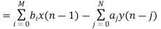
The direct form is obtained from

Based on the above equation, we need the current input sample and M−1 previous samples of the input to produce an output point. For M=5, we can simply obtain the following diagram from Equation 1.
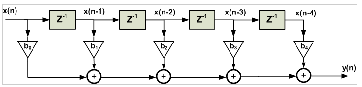
Fig 1 DF-1 Realization
On the other hand, for a linear-phase FIR filter, we observe the following symmetry in coefficients of the difference equation
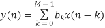
The structure obtained from the above equation is shown in Figure 2. While Figure 1 requires five multipliers, employing the symmetry of a linear-phase FIR filter, we can implement the filter using only three multipliers. This example shows that for an odd M, the symmetry property reduces the number of multipliers of an (M−1)th-order FIR filter from M to M+1/2.
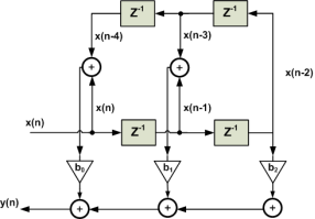
Fig 2 Final direct form structure
Cascade-Form Structure
The cascade structure is obtained from the system function H(z). The idea is to decompose the target system function into a cascade of second-order FIR systems. In other words, we need to find second-order systems which satisfy
where P is the integer part of M/2. For example, M=5, H(z) will be a polynomial of degree four which can be decomposed into two second-order sections. Each of these second-order filters can be realized using a direct form structure. It is desirable to set a pair of complex-conjugate roots for each of the second-order sections so that the coefficients become real.
Assume that we need to implement the nine-tap FIR filter given by the following table using a cascade structure.
k | 4 | 3 and 5 | 2 and 6 | 1 and 7 | 0 and 8 |
| 0.3333 | 0.2813 | 0.1497 | 0 | -0.0977 |

Solution:
The system function of this filter is

It can be show
Where

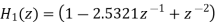
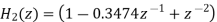
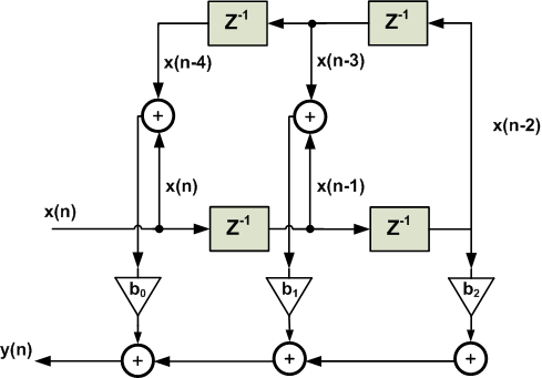
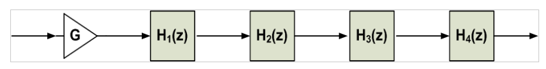
Fig 3 Cascade structure
Frequency-Sampling Structure
The frequency sampling method allows the use of recursive implementation of FIR Filter. There are two ways for frequency sampling
Non-Recursive frequency sampling filter
If the frequency shown below are sampled in the interval 0 to N-1 where N-1 is number of sampling. Sampling interval is Kfs/N, 0≤k≤N-1.
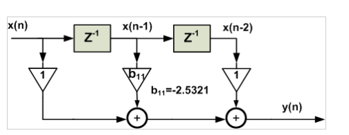
Fig 4 Frequency Sampling
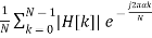
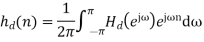
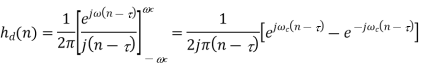
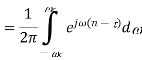
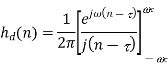
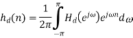
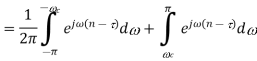
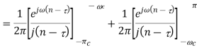
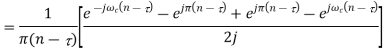
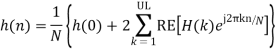
The FIR coefficient h[n] is calculated by IDFT of frequency samples.
h[n] = 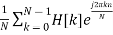 0≤k≤N-1.
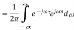
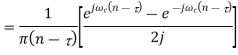
=

= 
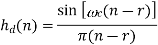
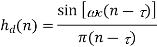
h[n] = 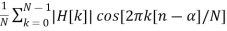
α = [N-1]/2
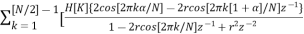
For N=odd, summation limit will be [N-1]/2
Recursive frequency sampling filter
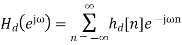
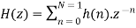
The recursive force of frequency sampling filter offers significant computational advantages over non recursive form if large number of frequency samples are zero valued. The transfer function of an FIR filter H[z] should be in recursive form. Impulse response of filter may be defined in terms of frequency samples.
h[n]= 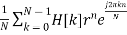
H[z]= 
Substituting value of h[n] and inter changing summation we have
H[z] = 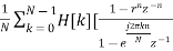 ]
]
H[z] can be represented as H[z] =H1[z]H2[z]
H1[z]=
H2[z] = 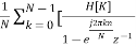 ]
]
Expanding above terms and solving them we finally get
H[z] = H1[z]H2[z]
H[z] = [
[
For frequency response we can replace z=ejωTs
H[ωn] = H[k] 0≤k≤N-1.
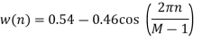
Key takeaway
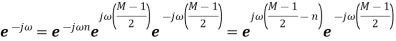
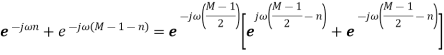
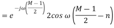
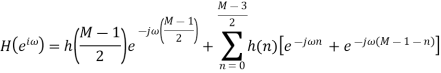
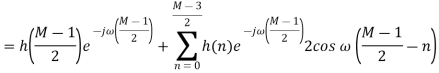
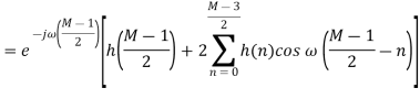
Linear phase is a property of a filter, where the phase response of the filter is a linear function of frequency. The result is that all frequency components of the input signal are shifted in time (usually delayed) by the same constant amount, which is referred to as the phase delay. And consequently, there is no phase distortion due to the time delay of frequencies relative to one another. Linear-phase filters have a symmetric impulse response. The FIR filter has linear phase if its unit sample response satisfies the following condition: h(n) = h(M − 1 − n) n = 0, 1, 2, . . . , N − 1 The Z transform of the unit sample response is given as
H[z] = 
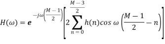
Symmetric impulse response with M=odd Then h(n) = h(M − 1 − n) and (z = ejω)

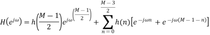


For M=even
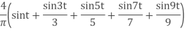
In practice it may be impossible to use all the terms of a Fourier series. For example, suppose we have a device that manipulates a periodic signal by first finding the Fourier series of the signal, then manipulating the sinusoidal components, and, finally, reconstructing the signal by adding up the modified Fourier series. Such a device will only be able to use a finite number of terms of the series.
Gibbs’ phenomenon occurs near a jump discontinuity in the signal. It says that no matter how many terms you include in your Fourier series there will always be an error in the form of an overshoot near the discontinuity.
The overshoot always be about 9% of the size of the jump. We illustrate with the example. of the square wave sq(t). The Fourier series of sq(t) fits it well at points of continuity. But there is always an overshoot of about .18 (9% of the jump of 2) near the points of discontinuity.
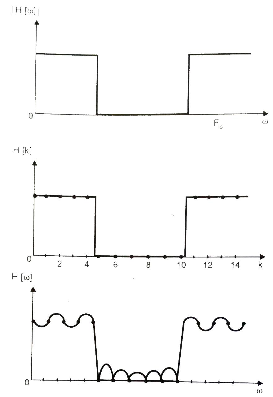
Fig 5 Gibbs Phenomenon
In these figures, for example, ’max n=9’ means we we included the terms for n = 1, 3, 5, 7 and 9 in the Fourier sum
Windowing method
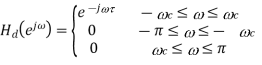
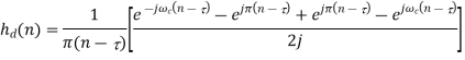
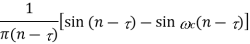
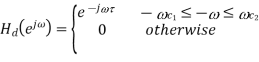
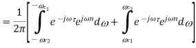
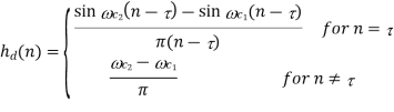
Let the frequency response of the desired LTI ststem we wish to approximate be given by
Where  is the corresponding impulse response.
Consider obtaining a casual FIR filter that approximates  by letting
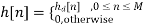
the FIR filter then has frequency response
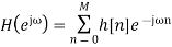
Note that sibce we can write
We are actually forming a finite Fourier series approximation to 
Since the ideal  may contain discontinuities at the band edges, truncation of the Fourier series will result in the Gibbs phenomenon.
To allow for a less abrupt Fourier series truncation and hence reduce Gibbs phenomenon oscillations, we may generalize h [n] by writing
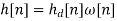
where  is a finite duration window function of length M +1.
Filter design using Kaiser window

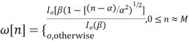
Where 
2. Choose  for the specified
  .
.
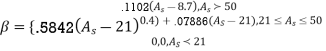
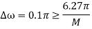
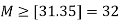
3. The window length M is then chosen to satisfy

4. The value for  is chosen as before
Note: Using the Kaiser empirical formula M can be determined over a wide range of  values to within
  . Very little if any literation is needed.
Design an FIR lowpass using the windowing method such that 
From the window characteristic we immediately see that for  Hammering window will work.
To find M set
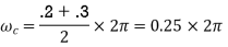
The cut-off frequency is
If a Kaiser window is desired, then for  choose

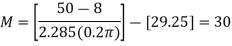
The prescribed value for M should be
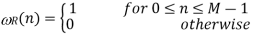
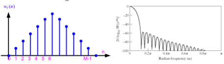
Rectangular Window
This is the simplest window function but provides the worst performance from the viewpoint of stopband attenuation. The width of main lobe is 4π/N
ωR(n) = 1 for n=0,1,M-1
= 0 otherwise
Magnitude response of rectangular window is
|WR(ω)| = 
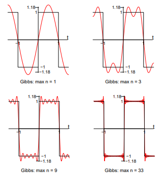
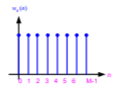
Fig 6 Rectangular Window
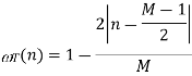
Bartlett (Triangular) Window
Bartlett Window is also Triangular window. The width of main lobe is 8π/M
ωt(n) = 1-
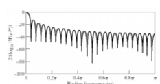
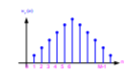
Fig 7 Bartlett Window
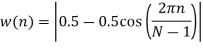
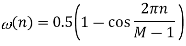
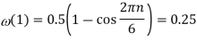
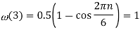
Hanning Window
This is a raised cosine window function given by:
W(n) = 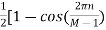 ]
]
W(ω) = 0.5WR(ω) +0.25[WR (ω - ) + WR (ω -
 )]
)]
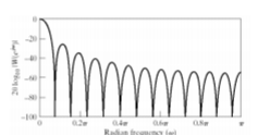
Fig 8 Hanning Window
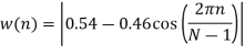
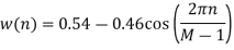
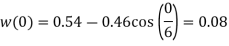
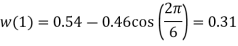
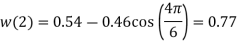
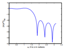
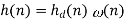
Hamming Window
This is a modified version of the raised cosine window
W(n) = 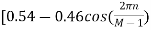 ]
]
W(ω) = 0.54WR(ω) +0.23[WR (ω - ) + WR (ω -
 )]
)]
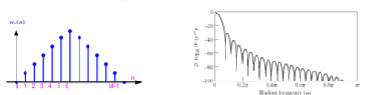
Fig 9 Hamming Window
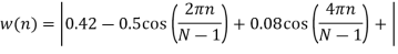
Blackman Window
This is a 2nd -order raised cosine window
W(n) = 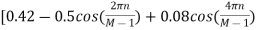 ]
]
W(ω) = 0.42WR(ω) +0.25[WR (ω - ) + WR (ω -
 )]+ 0.04[WR (ω -
 ) + WR (ω -
 )]
)]
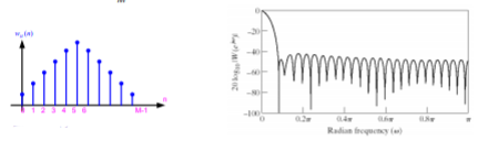
Fig 10 Blackman Window
Key takeaway
Window name
| Window function |
Rectangular |
|
Triangular
|
|
Hamming |
|
Hanning |
|
Blackman |
|
Window name | Transition width of main lobe | Min. stopband attenuation | Peak value of side lobe |
Rectangular |
| -21dB | -21dB |
Hanning |
| -44dB | -31dB |
Hamming |
| -53dB | -41Db |
Barlett |
| -25dB | -25Db |
Blackman |
| -74dB | -57Db |


Example
Q1) Design a LPF using rectangular window for the desired frequency response of a low pass filter given by ωc = π/2 rad/sec, and take M=11. Find the values of h(n). Also plot the magnitude response.
Sol:
r= M-1/2 = 5
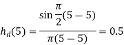
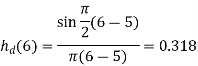
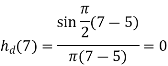
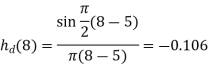
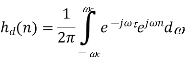
By taking inverse Fourier transform


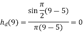
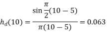
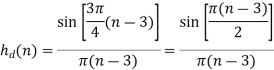
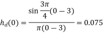
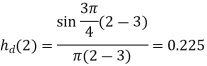
For  and
and 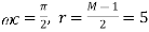
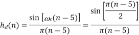
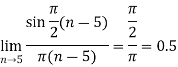
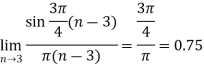
For 
 Using L’Hospital Rule

Where 
The given window is rectangular window ω(n) = 1 for 0 ≤ n ≤ 10
=0 Otherwise
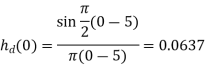
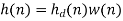
This is rectangular window of length M=11. h(n) = hd (n)ω(n) = hd (n) for 0 ≤ n ≤ 10
H[z]=  =
= 
The impulse response is symmetric with M=odd=11


|
|
|
|
|
|


Response
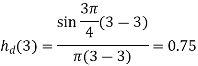
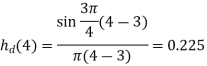
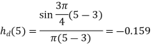
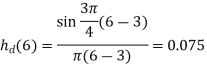
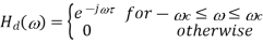
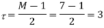
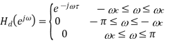
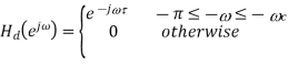
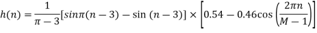
Q2) The desired frequency response of low pass filter is given by Hd (ejω) = e−j3ω − 3π/ 4 ≤ ω ≤ 3π/ 4 and 0 for 3π /4 ≤ |ω| ≤ π Determine the frequency response of the FIR if Hamming window is used with N=7
Sol
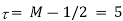
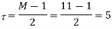
t = M-1/2 = 3


For  and
and 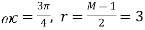
For 
 Using L’Hospital Rule
Where 

The given window is hamming window
To calculate the value of h(n)


The frequency response is symmetric with M=odd=7


|
|
|
|
|
|


RESPONSE
Q3) Design the FIR filter using Hanning window
Sol:


To calculate the value of 


Q4) Design an FIR filter (lowpass) using rectangular window with passband gain of 0 dB, cutoff frequency of 200 Hz, sampling frequency of 1 kHz. Assume the length of the impulse response as 7.
Sol:
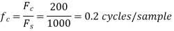


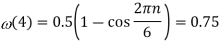
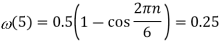
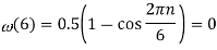
When 
When 
Calculating h(n)
As it is rectangular window h(n) = w(n)=hd(n)=h(n)
For M=7
n |
|
0 | -0.062341 |
1 | 0.093511 |
2 | 0.302609 |
3 | 0.4 |
4 | -0.062341 |
5 | 0.093511 |
6 | 0.302609 |

Q5) Using rectangular window design a lowpass filter with passband gain of unity, cutoff frequency of 1000 Hz, sampling frequency of 5 kHz. The length of the impulse response should be 7.
Sol:

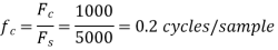


The filter specifications (ωc and M=7) are similar to the previous example. Hence same filter coefficients are obtained.
h (0) =-0.062341, h(1)=0.093511, h(2)=0.302609 h(3)=0.4, h(4)=0.302609, h(5)=0.093511, h(6)=-0.062341
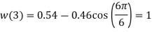
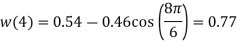
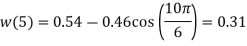
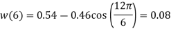
Q6) Design a HPF using Hamming window. Given that cutoff frequency the filter coefficients hd (n) for the desired frequency response of a low pass filter given by ωc = 1rad/sec, and take M=7. Also plot the magnitude response.
Sol:
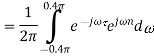
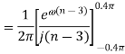
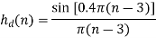
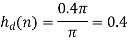
By taking inverse Fourier transform


The given window function is Hamming window. In this case
 for
for 
|
|
0 | -0.00119 |
1 | -0.00448 |
2 | -0.2062 |
3 | 0.6816 |
4 | -0.00119 |
5 | -0.00448 |
6 | -0.2062 |


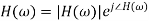
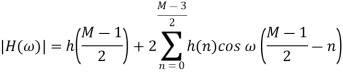
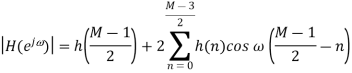
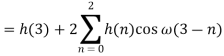
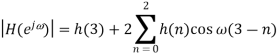
The magnitude response of a symmetric FIR filter with  is
is

For M=7


Q7) Design an ideal bandpass filter having frequency response Hde (jω) for π/ 4 ≤ |ω| ≤ 3π/ 4. Use rectangular window with N=11 in your design.
Sol:


The length of the filter with given is related by
And 
The given window is rectangular hence
for n=0,1,2,…,10 estimate the FIR filter coefficients h(n).
The frequency sampling method is use to design recursive and non-recursive FIR filters for both standard frequency selective filters and with arbitrary frequency response. The main idea of the frequency sampling design method is that a desired frequency response can be approximated by sampling it at N evenly spaced points and then obtaining N-point filter response.
A continuous frequency response is then calculated as an interpolation of the sampled frequency response. The approximation error would then be exactly zero at the sampling frequencies and would be finite in frequencies between them. The smoother the frequency response being approximated, the smaller will be the error of interpolation between the sample points.
There are two distinct types of Non-Recursive Frequency Sampling method of FIR filter design, depending on where the initial frequency sample occurred. The type 1 designs have the initial point at ω=0, whereas the type 2 designs have the initial point at f=1/2N or ω=π/N.
Procedure for Type I design


Desired filter coefficients
for linear phase filter with positive symmetrical impulse response,
4) take z transform of the impulse response h (n) to get the filter transfer function H (z)
Procedure for Type 2 Design
(Same steps as above expect step 2)
2) Samples  at N points by taking
 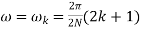 where
where 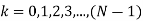 generate the sequence H (z)

Type 2 frequency samples gives additional flexibility in the design method to satisfy the desired frequency response at a second possible set of frequencies.
Key takeaway
There are two distinct types of Non-Recursive Frequency Sampling method of FIR filter design, depending on where the initial frequency sample occurred. The type 1 designs have the initial point at ω=0, whereas the type 2 designs have the initial point at f=1/2N or ω=π/N.
Direct-Form Structure
Direct form I
The difference equation


specifies the Direct-Form I (DF-I) implementation of a digital filter. The DF-I signal flow graph for the second-order case is shown in Fig.
Figure 11: Direct-Form-I implementation of a 2nd-order digital filter. |
Direct form II
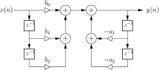
The signal flow graph for the Direct-Form-II (DF-II) realization of the second-order IIR filter section is shown in Fig.
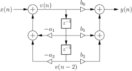
Figure 12: Direct-Form-II implementation of a 2nd-order digital filter
The difference equation for the second-order DF-II structure can be written as


which can be interpreted as a two-pole filter followed in series by a two-zero filter.
Signal Flow Graphs
A signal flow graph is a set of directed branches that connect at nodes. It provides the graphical representation of block diagram structure.
Fig 13 Representation of Branches and Nodes
The main points for SFG are listed below
Transposed Structure
Many times, it is required to transform one flow graph to another without changing basic input output relationship. Then we use trans position technique. It uses flow graph reversal theorem. The theorem stated that if we reverse the direction of all branch transmittances and interchange the input and output in the flow graph the system function remains unchanged. The resulting structure is called transposed structure.
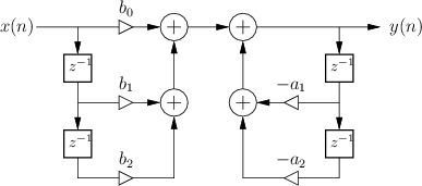
Fig 14 Transposed Structure
From above figure we can understand the concept. The above figure clearly shows that the role of adder and branching node is reversed. Now we draw the block diagram representation for the flow graph to get the transposed structure as shown in fig b.
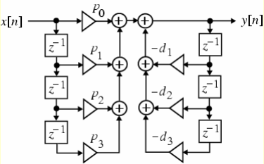
Cascade-Form Structure
The filter section can be seen to be an FIR filter and can be realized as shown below
W[n] = p0x[n] + p1x[n-1] + p2x[n-2] +p3x[n-3]
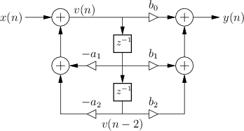
Fig 15 H1(z) realisation
The time-domain representation of H2(z) is given by
Y[n] = w[n] –d1y[n-1] –d2y[n-2] – d3y[n-3]
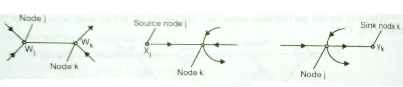
Fig 16 H2(z)
A cascade of the two structures realizing and leads to the realization of shown below and is known as the direct form I structure
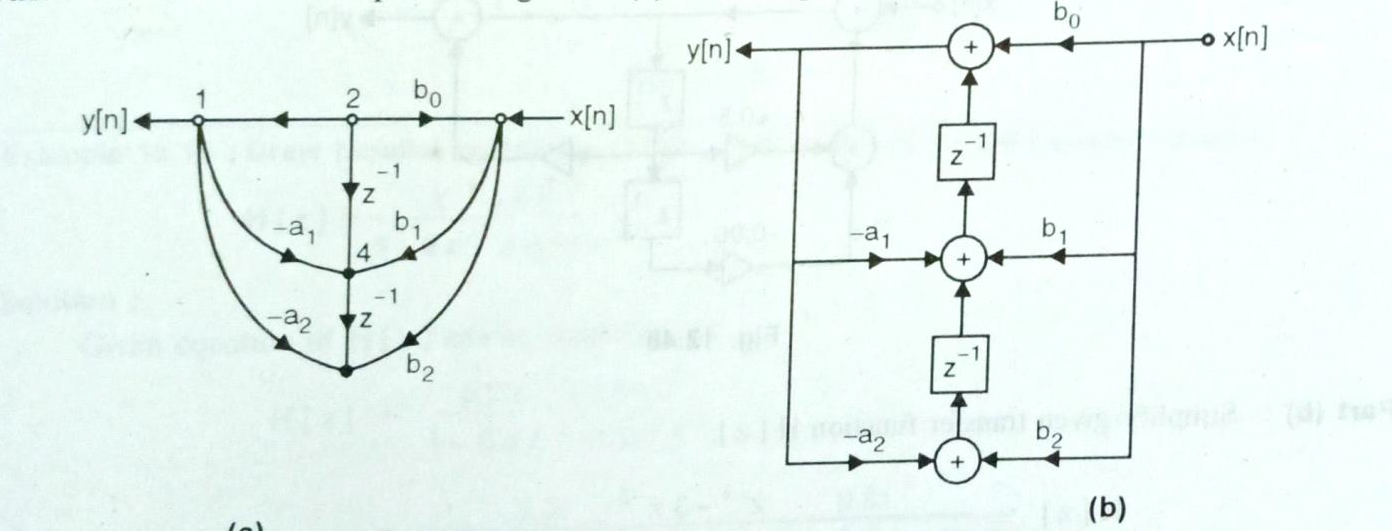
Fig 17 Cascade Realisation
Direct form II and cascade form realizations of
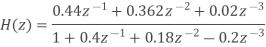
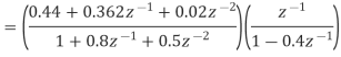
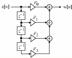
Fig 14 Direct form II
Fig 15 Cascade form
Parallel-Form Structure
Example. A partial fraction expansion of
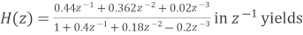
The corresponding parallel form I realization is shown below
Examples
Q1) Draw block diagram for the function using parallel form H(z)=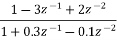
A1)
H(z)=
Writing above transfer function in standard form for parallel realisation we get
H(z)=-20+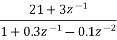
The structure is shown below
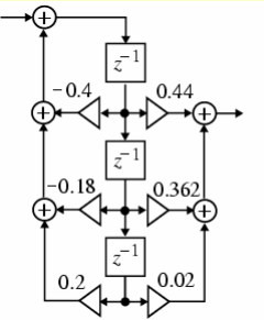
Fig 1 Parallel Realisation of H(z)=
Q2) For the following LTI system H(z)= . Realise the cascade form IIR filter.
A2) H(z)=
The above function can be simplified as
H(z)=
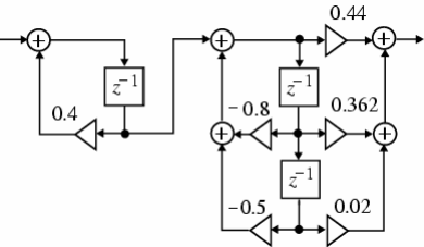
Fig 2 Cascade IIR Form
Hence, using the above structure and placing the values of 
 …. And similarly,
Q3) For the system given y(n) - y(n-1) +
  y(n-2) = x(n) +
  x(n-1) realise using cascade form?
A3) The system transfer function is given as
H(z) = Y(z)/X(z)
Taking z transform of y(n) - y(n-1) +
  y(n-2) = x(n) +
  x(n-1)
Y(z) -  z-1Y(z) +
  z-2 Y(z) = X(z) +
  z-1 X(z)
H(z)= 
Again, simplifying the above function to get into standard cascade form we ca write
H(z) = 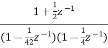
= H1(z)+H2(z)
H1(z)= 
H2(z)= 
The final structure is shown below
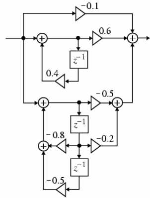
Fig 3 Cascade Form of H(z) = 
Q4) For the following LTI system H(z)= . Realise the cascade form?
A4) H(z)=
Writing the above in standard form for cascade realisation
H1(z)= 
H2(z)= 
The cascade structure is shown below
Fig 4 Cascade Form of H(z)=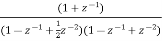
Q5) Realize the system transfer function using parallel structure H(z)= 
A5) H(z)= 
Taking Z common and then dividing the above function to convert it into standard form for parallel realisation we get
H(z)=Z [  +
+ +
+ ]
]
The parallel structure is shown below
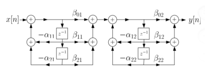
Fig 5 Parallel Realisation of H(z)= 
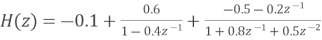
Q6) Realize the system transfer function using parallel structure H(z)= 
A6) Converting the above function to standard form using partial fraction technique
H(z)=  +
+ 
Solving for A and B we get
A= 10/3
B= -7/3
H(z) =  +
+ 
H1(z) = 
H2(z) = 
The parallel form realisation is shown below
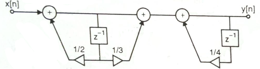
Fig 6 Parallel Realisation of H(z)= 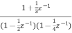
Q7) For the transfer function H(z) =  . Realise using cascade form?
A7) H(z) = 
Writing in standard form
H(z) = 
H1(z) = 
H2(z) = 
The cascade structure is shown below
Fig 7 Cascade Form of H(z) = 
Reference


