Unit - 2
Major methods for Measurement of stage
The maximum not unusual place technique utilized by the USGS for measuring speed is with a modern meter.
However, a number of superior systems also can be used to feel degree and degree stream flow. In the best technique, a modern meter turns with the go with the drift of the river or stream.
Stream flow is a size of the quantity of water flowing via a move or river over a set duration of time. Stream flow can't be measured directly, say, via way of means of plunging a device right into a river.
Instead, it should be calculated in a system referred to as move ganging. The USGS has been doing this seeing that 1889, while it set up its first move gage at the Rio Grande River in New Mexico to decide how an awful lot water turned into to be had for irrigation because the country extended westward.
Today, the USGS operates greater than 7,000 move gages throughout the U.S., which gives stream flow facts used broadly for flood prediction, water management, engineering and research, amongst different uses.
The USGS splits move gagging right into a three-step system: measuring move stage, measuring discharge and figuring out the stage-discharge relation.
Velocity:
Stream speed is the rate of the water within side the circulation. Units are distance in step with time (e.g., meters in step with 2d or toes in step with 2d).
Stream speed is finest in midstream close to the floor and is slowest alongside the circulation mattress and banks because of friction.
Velocity (v) is a vector amount that measures displacement (or alternate in position, Δs) over the alternate in time (Δt), represented via way of means of the equation v = Δs/Δt. Speed (or rate, r) is a scalar amount that measures the space traveled (d) over the alternate in time (Δt), represented via way of means of the equation r = d/Δt.
Stream flow:
Stream flow, or channel runoff, is the glide of water in streams, rivers, and different channels, and is a first-rate detail of the water cycle.
It is one issue of the runoff of water from the land to water bodies, the alternative issue being floor runoff. Water flowing in channels comes from floor runoff from adjoining hill slopes, from groundwater glide out of the ground, and from water discharged from pipes.
The discharge of water flowing in a channel is measured the use of movement gauges or may be envisioned through the Manning equation.
The file of glide over the years is referred to as a hydrograph. Flooding happens whilst the quantity of water exceeds the ability of the channel.
Sources of stream flow:
Channel precipitation is the moisture falling at once at the water floor, and in maximum streams, it provides little or no to discharge.
Groundwater, on the alternative hand, is a first-rate supply of discharge, and in huge streams, it bills for the majority of the common day by day glide.
Groundwater enters the streambed wherein the channel intersects the water table, presenting a consistent deliver of water, termed base flow, in the course of each dry and wet periods.
Because of the huge deliver of groundwater to be had to the streams and the slowness of the reaction of groundwater to precipitation events, base flow adjustments simplest steadily over time, and it's far not often the principle reason of flooding.
However, it does make contributions to flooding via way of means of presenting a degree onto which runoff from different re assets is superimposed.
Interflow is water that infiltrates the soil after which actions laterally to the circulate channel within side the sector above the water table. Much of this water is transmitted in the soil itself, a number of it shifting in the horizons.
Next to base flow, it's far the maximum essential supply of discharge for streams in forested lands. Overland glide in closely forested regions makes negligible contributions to stream flow. In dry regions, cultivated and urbanized regions, overland glide or floor runoff is often an essential supply of stream flow. Overland glide is a storm water runoff that starts as skinny layer of water that actions very slowly (generally much less than 0.25 ft consistent with second) over the ground. Under in-depth rainfall and within side the absence of limitations consisting of difficult ground, vegetation, and soaking up soil, it could mount up, swiftly accomplishing circulate channels in min s and inflicting unexpected rises in discharge.
Key takeaways:
The dating or relations ship among the quantity of water flowing in a river or circulation and degree at any precise factor is generally referred to as degree–discharge dating
The level-discharge relation—defining the herbal however regularly converting relation among the level and discharge; the usage of the level-discharge relation to transform the constantly measured level into estimates of stream flow or discharge
Discharge Rating' is usually defined as the relation between the river level and discharge. The terms 'score', 'score curve', 'station score', and 'level-discharge relation ' are synonymous with the term 'discharge score'.
The measured discharge is plotted against the corresponding level to define the score curve; the plot could be in square coordinates or logarithmic. The discharge is plotted because the abscissa and the level because the ordinate in square coordinates.
While it's far lots simpler to examine the degrees of a river, the release statement by truly measuring the intensity and pace of the go with the drift is bulky and expensive. Hence the facts are frequently accumulated within side the shape of degrees and is transformed into discharge with the help of a longtime level-discharge relation because the facts within side the shape of discharge can be more meaningful and desired by the users in their analysis.
A good and stable level- discharge relation is very lots essential for estimating the discharges accurately from the observed degrees.
Though the World Meteorological Organization (WMO) recommends a minimum of ten discharge measurements per year, it may be necessary to have regular daily observations of level and discharge concurrently for a preliminary length with a purpose to establish a dependable level- discharge relation at a hydrological statement station.
The SCS curve quantity approach is a simple, broadly used and green approach for figuring out the approxient quantity of runoff from a rainfall even in a selected area. Although the approach is designed for an unmarried typhoon event, it may be scaled to locate common annual runoff values.
When the facts of accumulated rainfall and runoff for long-duration, high-intensity rainfalls over small drainage basins are plotted, they display that runoff best begins off evolved after a few rainfall has accumulated, and that the curves asymptotically method a straight line with a 45-diploma slope.
The Curve Number Method is primarily based totally on those two phenomena. The initial accumulation of rainfall represents interception, depression storage, and infiltration before the begin of runoff and is called initial abstraction.
After runoff has started, a number of the extra rainfall is lost, specifically within side the shape of infiltration; that is called real retention.
With increasing rainfall, the real retention also increases up to a few most value: the capability most retention.
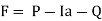
To describe those curves mathematically, SCS assumed that the ratio of real retention to capability most retention became same to the ratio of real runoff to capability most runoff, the latter being rainfall minus initial abstraction. In mathematical shape, this empirical courting is

Where,
I, = initial abstraction (mm)
T he above courting for sure values of the preliminary abstraction and potential maximum retention.
After runoff has started, all additional rainfall turns into both runoff or actual retention (i.e., the actual retention is the difference among rainfall minus preliminary abstraction and runoff).
Key takeaways:
Flow mass curve:
The mass curve technique, proposed through Ripple in 1883 to decide garage capability of a reservoir, is a graphical technique.
To decide minimal required garage, the mass curve of influx and the mass curve of call for are gathered separately.
The line AB is the mass curve of demands.
As we have already seen that the storage capacity of any reservoir depends upon the nature of the inflow the amount of water received from the inflow, depth of the reservoir the rock strata around the reservoir climatic conditions (to determine the rate of evaporation) etc.
It is necessary to calculate the capacity reservoir to meet the demand of water for various purposes.
This capacity of the reservoir can be determined by the Mass curve and the demand curve as explain below:
Use of Mass Curve to Determine the Capacity of the Reservoir:
The span of the period to be considered, must have a critical or driest period of the region (which would) indicate the lower most figures of the stream inflows look at the Fig. which has expressed a mass curve for period of six years. Le from the year 2000 to 2006
2. The time period in years in given an x axis and the accumulated flow is given on y axis. In this Fig. in the downward side, the demand curve has been drawn (for the comparison).
It indicates the variation in the rate of demand. If the rate of demand is constant, the demand curve will be a straight line (with no curve) the demand curve is always on rise as the population nesses, the consumption of domestic purpose, irrigation purpose, industrial purpose, hydel power generation purpose always increases
3. On the A-B curve, G-H, and F-J doted lines are drawn, parallel to the demand curve and are tangent to the high points like, G and H of the mass curve. These are the point placed at the beginning of the dry period.
4. In the mass curve, maximum vertical intercepts i.e., x₁ y₁, X₂ Y₂ etc. between the tangential lines are drawn to measure the mass curve. These vertical intercepts i.e., x, y, or x, y, indicate, the volume by which the total inflow of the stream falls short of the demand and so it is necessary to make supply form the reservoir storages. (Refer Fig.)
Let us assume that the reservoir to be fall at point G (in the Fig. 5.4.1) for a period from G to Z, (in the year between 2001 and 2002) there is a total inflow in the stream which is represented by Y, Z, and at the same time the total demand is represented by X, Z, (leaving a gap of volume of water, shown by X, Y,). This is needed to be met by using reservoir's storage.
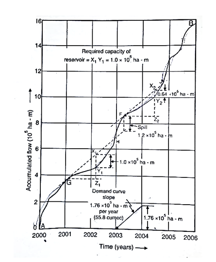
5. The largest of the maximum vertical intercepts i.e., X, Y, X, Y, etc.; represent the capacity of the reservoir, required to satisfy the given demand.
Whatever has been calculate in the 'Net storage' required to meet the demand, so if there is any type of evaporation or percolation loss in the storage of the reservoir, it must be compensated by using storage capacity.
The vertical distance between two tangential lines, such as GH and FJ, represents the extra amount of water which spills over from the reservoir, through the spillway.
It goes as a waste in the dam stream direction. This happens because between height of H and F, the reservoir remains full and so all the inflow in excess of demand will be sent out through the spill way to the downstream side.
If these tangential lines which are drawn parallel to the demand curve, are extended further, they should intersect' the mass curve e.g., at H or J. so the reservoir which was full at G and F will be filled soon, but these extended lines do not intersect the mass curve it will indicate that the reservoir will not be filled again.
If the reservoir is very large, the time interval between the points G and H; F and J etc. may be of several years.
Key takeaways:
1. Hydrographs Components:
It has three components as shown below
a) The Rising curve
b) The crest (The Peak point)
c) The falling curve.
Hydrograph is a graph that shows the discharge i.e., the rate of flow of surface water versus the time past a specific point in a stream or a river.
The rate of flow is expressed in cubic meters per second (cms).
As shown in Fig. The hydrograph has rising curve / rising limb peak discharge / the crest and the falling curve/falling limb.
(A) The rising curve/Rising limb:
It is also called as concentration curve. It reflects the prolonged rise in the discharge, from the catchment; with the result of the rainfall.
(B) The peak discharge / The crest:
It is the highest point of the Hydrograph to indicate the maximum discharge per sec.
(C) The falling curve / Falling limb:
It extends from the crest to indicate the end of the storm flow. This curve represents the withdrawal of water from the storage built up in the basin during the earlier phases of the hydrograph.
2. Affecting factors of hydrograph:
1) Shape
A round fashioned drainage basin results in speedy drainage while an extended drainage basin will take time for the water to attain the river.
2) Topography & relief
The steeper the basin the extra quick it drains. Indented landscapes will accumulate water and decrease runoff rates, lowering the quantity of water achieving the river channel.
3) Heavy Storms
Runoff will boom after soil area capability is met this means that water will attain the channel quicker.
4) Lengthy rainfall
This results in the floor being saturated and runoff will boom this means that water will attain the channel extra quick as soon as soil capability has been reached.
Snowfall until the snow melts, the water is held in garage however while the snow melts this may cause flooding.
5) Vegetation
This can lessen discharge because it intercepts precipitation. Roots of vegetation also can soak up water that is going into the soil.
Seasonally, within side the UK the flora will lessen discharge within side the summer time season while within side the wintry weather it's going to have much less of an effect because of much less foliage being gift on trees.
6) Rock type
The underlying geology varies inside drainage basins and may be permeable (permitting water through) or impermeable (now no longer permitting water through). Impermeable rocks inspire more quantities of floor runoff and an extra speedy boom in discharge than permeable rocks.
3. Base flow separation methods:
The base flow is a portion of the stream for which is not directly generated from the excess rainfall during the storm event.
To separate the base flow the straight-line method is commonly used. It is useful for an individual steam i.e., a single storm only.
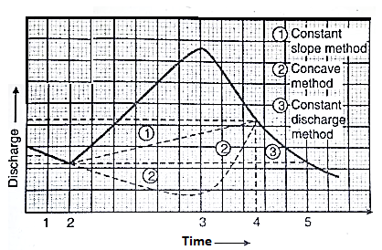
Other method of Base flow separation is
(1) Constant-slope method
(2) Concave method
(3) Constant discharge method
Key takeaways:
1. Unit hydrograph:
Unit hydrograph can be defined as, "a method to express the relation; between time and the discharge by graphical method".
The units of time are hours, days or months which are expressed on the X-axis as per the requirement i.e., the unit of time depends upon the purpose and nature of study e.g.
If the study is confined to the discharge of water through floods the unit will be hours and in case of discharge through run off is to be calculated the unit will be either a month or a year.
The discharge is expressed by m³/s. In some cases, the discharge is expressed in cm/s i.e., depth of the case of water per unit are of the catchment, per second e.g., cm/s/m².
To develop, the theory of unit hydrograph, the following definitions are taken as the base.
a) Excess Rainfall unit
It is total precipitation after all the abstractions like evaporation, infiltration, surface storage and interception.
Excess rainfall is 1 unit. It may be 1 cm or 4 cm. let is imagine that the excess rainfall unit is 1 cm, so the excess rainfall will be 1 cm /n for 1 hour or 1/2 cm / h for 2 hours; or 2 cm /n for 1/2 hour.
b) Duration of Excess Rainfall
This duration must be lesser than the period of concentration i.e. [The base period of T is the total time of flood hydrograph at a given gauging site.]
Specifications of Unit Hydrograph
Both the, unit of precipitation and the intensity of the excess precipitation are the controlling parameters.
So, in case of unit hydrograph, it is specified as 1 cm 1 h hydrograph (in this unit if precipitation is 1 cm and period of precipitation is 1 hour so, intensity of the precipitation will be 1 cm / n). e.g., The surface runoff a catchment area of A km² will be; Surface Runoff = (1 cm / 100) x A x 10 m³ = (A / 100) × 10 m³ = A x 10¹ m³
Assumption:
2. Derivation:
Unit hydrograph can be derived from the Observed hydrograph.
Rainfall and its Resultant before doing so, it is always necessary to scan the data, which has been made available.
The step-by-step procedure is as given below. An isolated storm and its resultant hydrograph from the observed data must be selected.
3. Uses of hydrographs:
The hydrographs have the following uses:
(A) They help to know the magnitude of the extreme rainfall.
(B) They help to decide the design of the hydraulic structure.
(C) They are useful in extension of flood flow records (based on rainfall records)
(D) They are very useful for the development of flood forecasting and flood warning system to reduce the losses due to floods.
4. Limitations of Unit Hydrograph:
1. The basic assumption of uniform distribution of the excess rainfall over. The entire catchment is far away from the reality.
2. The principle of linearity is assumed in this theory, which, in reality is not correct. This theory is not applicable to the surface runoff originated form show and Ice.
3. The theory is applicable for the floods in bank only i.e., the flood water is contained to the river channel only. It is not applicable in the areas where the floods over cross the banks.
4. The theory is applicable to the catchment area which is less than 5000 km², only.
5. The theory is not applicable to the narrow-elongated catchments because in such cases the uniform distribution of the perception is not possible over the entire catchment area.
6. The theory becomes un applicable in the catchment having surface storages in the upstream areas of the gauging station.
Key takeaways:
Flooding is the worst weather-associated hazard, inflicting lack of lifestyles and immoderate belongings harm.
In general, flash floods are characterized through their speedy onset, leaving very constrained powerful reaction opportunities.
Flood harm mitigation is furnished via a number of structural and nonstructural methods. A widespread nonstructural approach is the operation of flood caution systems. Currently, 3 standards are used for an anticipated flooding determination: crucial discharge, crucial runoff, and crucial rainfall (CR). Critical rainfall criterion is utilized by maximum flood caution systems.
Given a preliminary soil moisture circumstance and a rainfall duration (D), exceptional hyetographs display the numerous areal rainfall volumes over the take a look at basin important to motive minor basin outlet flooding that is described as threshold rainfall (TR), and the minimal of those TR values is known as CR. That is to say, TR is a characteristic of preliminary soil moisture circumstance, rainfall duration, and the shape of rainfall hyetograph, however CR is a characteristic of simplest preliminary soil moisture circumstance and rainfall duration.
No remember whether or not an inverse or wonderful technique is used, TR values are constantly computed with the aid of using routing floor runoff the usage of the UH technique.
So, deriving the UHs representing the authentic basin attention traits is a key to calculating the CR estimate matching the minor rainfall price vital to motive flooding. For extra than seventy-five years for the reason that inception of UH principle changed into provided with the aid of using Sherman, it's far nevertheless one of the maximum broadly used strategies for flood prediction and caution gadget improvement in gauged basins with discovered rainfall and runoff data, however this data-pushed conventional method limits the UH derivation handiest to gauged watersheds.
Synthetic UHs can also additionally handiest be utilized in basins whose hydrographs have an unmarried peak.
Geomorphologic UHs, irrespective of time-invariant (TIVUH) or time-variant (TVUH) do now no longer take the dynamic factor (glide speed) spatial distribution into account.
Distributed UHs primarily based totally on a spatially disbursed speed area can safely take the non uniformity of basin traits into account.
Formulas described as a characteristic of rainfall depth are followed to compute spatially disbursed speed fields so that it will derive TVUHs that may remedy to a positive quantity the nonlinear trouble of runoff attention.
Key takeaways:
1. Peak flood estimation by rational method:
It is a method derivation of design flood from storm studies and application of unit hydrograph principle
In this method following steps are taken,
(i) Analysis of rainfall v/s runoff date for derivation of loss rate under the critical conditions.
(ii) Derivation of unit hydrograph by analysis (if the data are not available by synthesis).
(iii) Derivation of design storm.
(iv) Derivation of design flood, from the design storm (by applying the rainfall, excess increment to the unit hydrograph)
In the regions, having snowfall, this unit hydrograph principle is not useful.
2. Empirical formulae:
These formulae are based on the actual field data wherein following parameters are considered,
Following formulae are used to calculate the rainfall - runoff relationship.
He has suggested two formulae, based on the field observations of two different geographical locations, in the old Bombay State. They are as follows:
Ghats fed Catchments [i.e., The western slopes of western Ghats receiving heavy rains from the south west monsoon winds]
R = 0.85 P-30.5
Plain areas in water-shadow regions [i.e., The Eastern slopes of Western Ghats, receiving less rainfall as they are on the Lee-ward side of the Western Ghats].
R = Px(P-17.8) 2.54
Where in, R = Runoff, (in mm);
P = Precipitation (in mm)
If a catchment area has some parts in Ghats region and some in plain rain shadow region use both the formulae separately to calculate the runoff and then add these two figures to get the total runoff of that catchment area.
B. Khosla's Formula
In his formula, Dr. Khosla has added one more aspect of temperature to see the effect of evaporation on the total water received through the precipitation. The formulae read as, R = P-ST
Where,
R = Runoff (in mm);
P = Average Precipitation (in mm)
T = Average temperature (in 0¹)
Using the above formula for each month, monthly average runoff is calculated and all the values of twelve months are added together to get annual runoff.
If the average temperature is less than 10°C, the formula is modified.
3. Enveloping curve:
In this, the maximum flood is obtained from the envelope curve of all the maximum observed floods, for a number of catchment areas, in a region where in theme is a homogeneity in the climatic conditions and the numerical values are plotted against the drainage area.
This method is useful for the generalizing the limit of the floods.
4. Gamble’s method:
Gamble’s felt that the distribution of the flood is unlimited and there is no chance to impose any physical limit to the maximum or peak floods
So, he has advocated that the possibility Lc. the Probability (P) of the occurrence of a flood of values or magnitude will be equal or exceed than any specified value (x), can be expressed by the following equation
In this
e= the base of the Natural logarithms and
a= the reduced variant as given in the following equation:
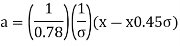
Where,
X = The magnitude of the flood of probably (P)
X = Arithmetic mean or the average of the floods in the assumed series
 = The standard deviation fort this flood series.
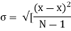
Where,
N = The total number of items in the flood series. (The number of years for which the record of flood exists)
The recurrence interval (T) can then be calculated by making the use of, T, =
The various values of the reduced variates (b) which are corresponding to the values of return period (T) and the probability exceedance are given in the standard tables.
Frequency factor of gamble’s method:
The general principle of frequency analysis can be stated as
The frequency i.e., the probability P (X ≥ x) of the observed flood peaks can be calculated. The curve of the probabilities versus flood peaks [F vs X].
It is then plotted, on a log-probability paper and a smooth curve is fitted by covering all the points. [By extrapolation of the curve the extreme values are obtained]
As, generally the observed data is short we cannot keep entire reliance on the curve based on the observed data.
Gambel's method of frequency analysis is based on the extreme value distribution and uses the frequency factors which are developed for the theoretical distribution.
Key takeaways:
References:


