Unit 1
Heat Conduction
The process of heat transfer takes place through 3 distinct modes: Conduction, Convection and radiation.
1.2.1 Conduction
The mechanism of heat transfer due to temperature gradient in a stationary medium is called conduction. The medium may be solid or fluid. In fluids, conduction is due to collision of molecules in the course of their random motion. In solids, conduction is attributed to:
Fourier’s law of heat conduction states that the rate of heat transfer is linearly proportional to the temperature gradient. For one-dimensional or unidirectional heat conduction

 ..(1.1)
where, qk is the rate of heat flux (a vector) in W/m2, dT/dx is the temperature gradient in the direction of heat flow x and k is the constant of proportionality, which is a property of the material through which heat propagates. This property of the material is called thermal conductivity (W/m K).
1.2.2 Convection
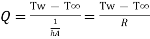
It states that rate of heat transfer is proportional surface area perpendicular to heat flow direction and temperature difference between wall surface (Tw) and fluid temperature (T∞) in direction perpendicular to flow.
 Tw - T∞)
 Tw - T∞) ..(1.2)
Where, Q is rate of heat transfer (W), A is area in m2, h is constant known as coefficient of convective heat transfer or film coefficient with unit W/m2K.
1.2.3 Radiation
 ..(1.3)
Where,  is the Stefan-Boltzmann constant, 5.67 X 10⁻⁸ W/m2 K4.
Let us consider an infinitesimal volume element of side dx, dy and dz (Fig. 1.1). The considerations here will include the non-steady condition of temperature variation with time t.
Let T be temperature at the center of element.
Let the material be anisotropic, hence thermal conductivities have different values kx
ky and kz in x,y and z direction respectively.
Consider heat leaving and entering this volume through six faces.
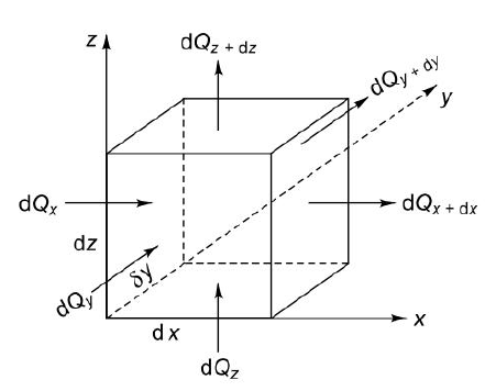
Fig. 1.1 Volume element for determining heat conduction equation
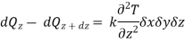
According to the Fourier heat conduction law, the heat flowing into the left-most face of the element in the x-direction

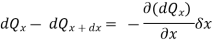
The value of the heat flow out of the right face of the element can be obtained by expanding dQx in a Taylor series and retaining only the first two terms as an approximation:

The net heat flow by conduction in the x-direction is therefore
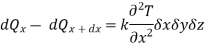
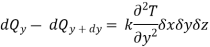
Similarly,
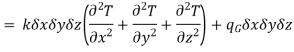
Here, the solid has been assumed to be isotropic and homogeneous with properties uniform in all directions. Let us consider that there is some heat source within the solid, and heat is produced internally as a result of the flow of electrical current or nuclear or chemical reactions. Let qG is the rate at which heat is generated internally per unit volume (W/m3). Then the total rate of heat generation in the elemental volume is

The net heat flow owing to conduction and the heat generated within the element together will increase the internal energy of the volume element. The rate of accumulation of internal energy within the control volume is

where c is the specific heat and  is the density of the solid.
An energy balance can be achieved on the volume element as:
Rate of energy storage within the solid = Rate of heat influx – Rate of heat outflux + Rate of heat generation
Or

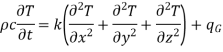
…(1.4)
where  is the thermal diffusivity of the solid given by
  k/
k/ . The larger the
value of  , the faster heat will diffuse through the material.
This is heat balance equation in Cartesian form.
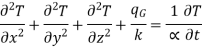
If the temperature of a material is not a function of time, the system is in the steady state and does not store any energy. The steady state form of a three-dimensional conduction equation in rectangular coordinates is
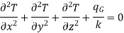
…(1.5)
It is known as Poisson’s equation.
If the system is in steady state and no heat is generated internally, the conduction equation further simplifies to
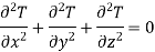
…(1.6)
This is known as Laplace equation.
Consider heat flow in x-direction only with no heat generation. Hence Laplace equation reduces to

…(1.7)
This equation is known as one dimensional heat conduction equation with no heat generation.
1.3.1 Heat conduction equation in cylindrical co-ordinates
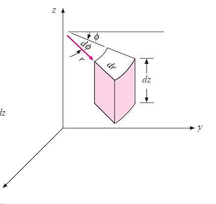
Fig 1.2 Heat conduction in cylindrical element
For a general transient three-dimensional heat conduction problem in the cylindrical coordinates with T = T (r, q, z, t)
By substituting x=rcos , y=rsin
 and z=z equation (1.4) becomes
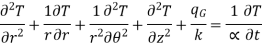
…(1.8)
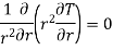
Considering material as isotropic and heat transfer occurring to be one dimensional in steady state equation reduces to

…(1.9)
This equation is known as one dimensional heat conduction equation with no heat generation in cylindrical co-ordinate system.
1.3.2 Heat conduction equation in spherical co-ordinates
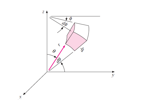
Fig 1.2 Heat conduction in spherical element
Consider a spherical element with co-ordinate (r, ,
, )
)
Substitute 

…(1.10)
Considering material as isotropic and heat transfer occurring to be one dimensional in steady state equation reduces to
This equation is known as one dimensional heat conduction equation with no heat generation in spherical co-ordinate system.

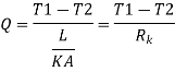
Where Rk=L/KA is conductive thermal resistance offered by thermal wall.
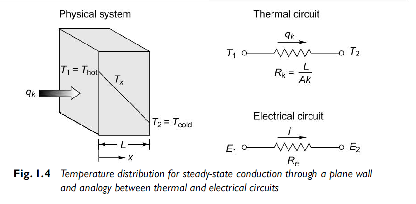
1.4.1 Heat transfer in plane wall
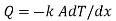
From Fourier law, 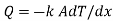
From fig1.4, at x=0, T=T1
At x=L, T=T2
On integrating, 
Conductive resistance R=
1.4.2 Heat transfer by convection
By Newton’s law 
Where R= is a convective resistance.
1.4.3 Overall heat transfer coefficient
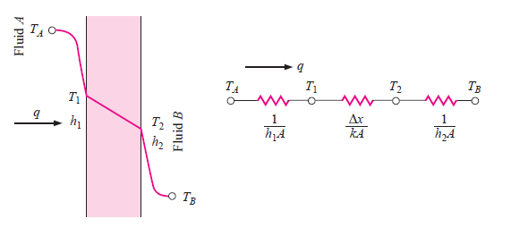
Fig.1.5 Overall heat transfer through plane wall
Consider the plane wall shown in Figure 1.5 exposed to a hot fluid A on one side and a cooler fluid B on the other side. The heat transfer is expressed by
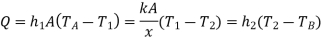
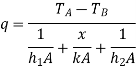
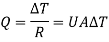
The heat-transfer process may be represented by the resistance network in Figure 1.5, and the overall heat transfer is calculated as the ratio of the overall temperature difference to the sum of the thermal resistances
The overall heat transfer by combined conduction and convection is frequently expressed in terms of an overall heat-transfer coefficient U, defined by the relation

Where A is area of heat flow and
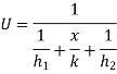
…(1.11)
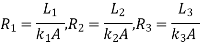
1.4.4 Resistances connected in series
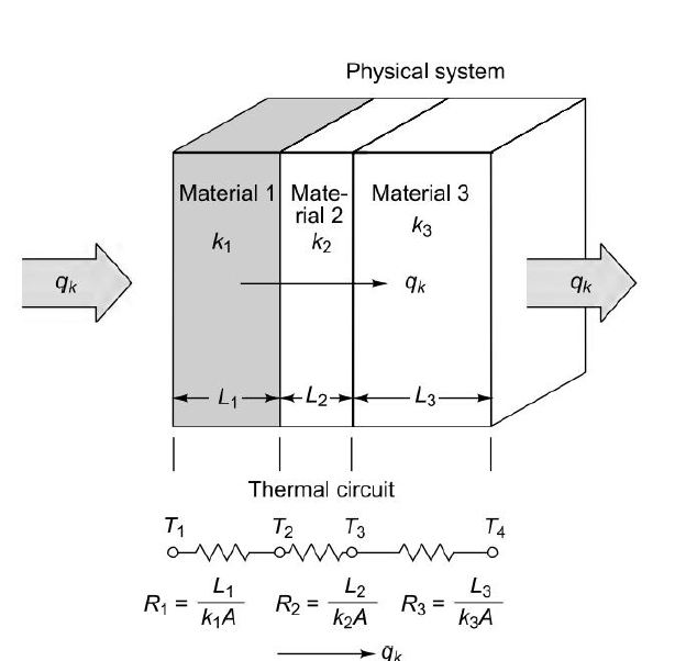
Fig1.6 Conduction through three resistances in series
Consider 3 slabs connected in series with endpoints insulated to avoid loss of heat due to convection. This system is equivalent to electric system. Hence,

1.4.5 Resistances connected in parallel
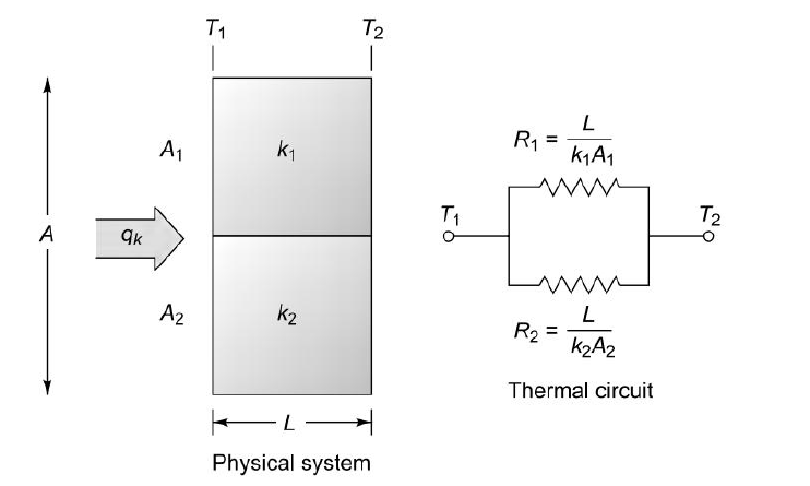
Fig1.7 Conduction through three resistances in parallel
Consider 2 slabs connected in parallel with endpoints insulated to avoid loss of heat due to convection. This system is equivalent to electric system connected in parallel. Hence,

 ,
,
Therefore, 
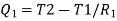
1.5.1 Heat transfer through infinitely long hollow cylinder
Fig 1.8 Heat transfer through infinitely long hollow cylinder
Consider a hollow cylinder of internal and external radius r1 and r2 with respective internal and external temperatures Ti and To. Let L be length of cylinder and k be thermal conductivity. Heat transfer takes place radially. Consider a ring of radius r and thickness dr. From Fourier’s law

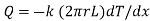
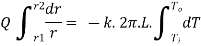
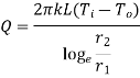
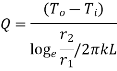
…(1.12)
where , represents thermal resistance.
1.5.2 Heat transfer through hollow sphere
Consider a hollow sphere of internal and external radius r1 and r2 with respective internal and external temperatures Ti and To. k be thermal conductivity. Heat transfer takes place radially. Consider a ring of radius r and thickness dr.
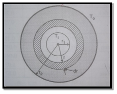
Fig 1.9 Heat transfer through infinitely long hollow sphere
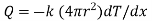

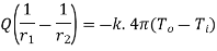
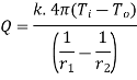
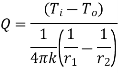

…(1.13)
Where  represent thermal resistance.
1.6.1 Critical radius of insulation in cylinders
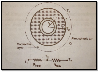
Fig 1.10 Critical thickness of cylinder
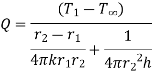
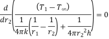
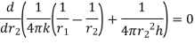
Consider heat flow from metal tube of outside radius r1.It is insulated by layer of insulation with outer radius r2. Let temperature of outside surface of metal tube is T1, conductivity of insulation be k(W/m K). Insulation is exposed to atmosphere at temperature T∞ with convective heat transfer coefficient h(W/m2K) and length L in meters. Now the heat transfer rate through metal tube is
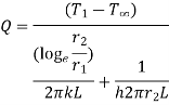
…(1.14)
From above equation, it can be seen that with increase in insulation ( heat flow rate Q may decrease or increase with increase in
  since conductive resistance
  increase logarithmically but conductive resistance
  decrease linearly.
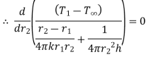
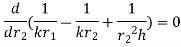
To find value of  for which Q is maximum
  should be equated to zero. Hence differentiating 1.14 with respect to
  and equating equal to zero.
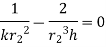
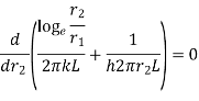
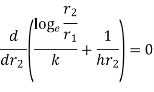
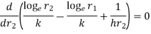
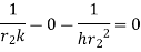


…(1.15)
Where  is critical radius of insulation.
Therefore, at  heat loss will be maximum.
At  , heat transfer will increase until
  increases and becomes equal to
  .
.
If  , heat transfer will go on decreasing and insulation effect will be achieved.
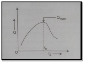
Fig1.11 Variation of heat transfer with insulation radius
1.6.2. Critical radius of insulation of Sphere
Consider a hollow sphere with outer radius r1 at temperature T1 which is covered with insulation of outer radius r2. Insulation is exposed to atmosphere at temperature T∞ with convective heat transfer coefficient h(W/m2K). Let temperature of outside surface of metal sphere is T1, conductivity of insulation be k(W/m K).
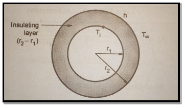
Fig 1.12 Critical thickness of sphere
From 1.13 ,
For maximum heat transfer,
Differentiating denominator for it’s minimum value

…(1.16)
1.16 is equation for critical radius of insulation for sphere.
Variation in heat transfer with change in radius in insulation is same as of cylinder.
Convection heat transfer between a surface (at T1) and the fluid surrounding it (at  ) is given by
where h is the heat transfer coefficient and A is the surface area of heat transfer.
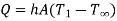
Consider a plane wall. If T1 is fixed, the heat transfer rate may be increased by increasing the surface area across which convection occurs. This may be done by using fins that extend from the wall into the surrounding fluid.
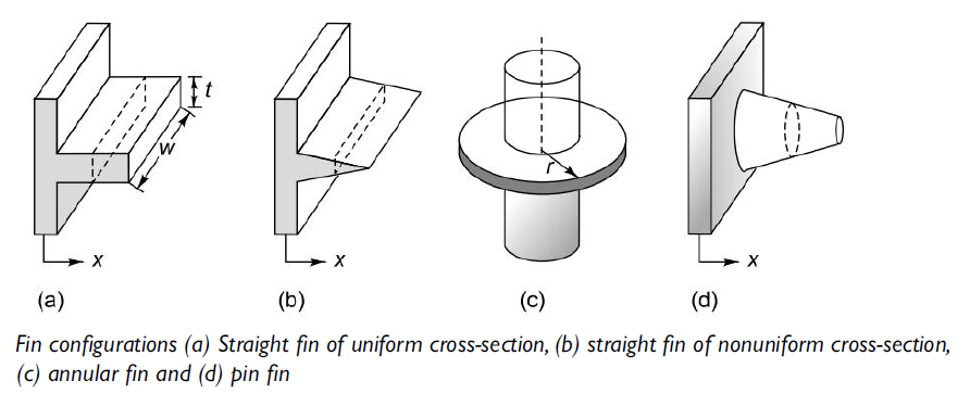
Fig 1.13 Types of Fins
1.7.1. Analysis of fin of uniform cross-section area(pin-fin)
Consider a thin rectangular fin of uniform cross-section. The fin is attached to base surface at temperature To. Let Ac be cross-sectional area and P be perimeter of fin, is atmospheric temperature and L is length of fin. Following assumptions are made in this analysis:
Heat is conducted from base surface to fin by conduction and from fin to atmosphere by convection simultaneously.
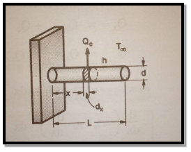
Fig 1.14 Pin fin
Consider a element section of thickness dx at distance x from base. Let T be be temperature at section.
Heat entering in elementary section,

Heat conducted out from element
Heat convected out of element through thickness dx
By energy balance equation,
Heat conducted into element = Heat conducted out + Heat convected out
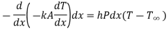
…(1.17)
Let  and
and  By differentiating

And

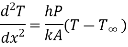
Hence 1.17 becomes

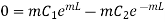
Above equation is second order differential equation. General solution for this equation is

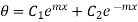
…(1.18)
And slope is

…(1.19)
In order to find solution of above differential equations we need values of  and
and  . We can obtain solution for following three cases:
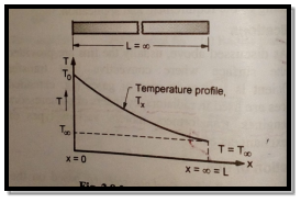
Fig 1.15 Infinitely long fin
Consider a infinitely long fin as in figure such that temperature at the end of fin approaches surrounding temperature  .
.
At  hence
hence  .
.
At 
Applying boundary condition 1 to 1.18

…(1.20)
Applying boundary condition 2 to 1.18
Hence  . Putting this value in 1.20
Substituting values of  and
and  in 1.18
…(1.21)

…(1.22)
This represents temperature distribution on infinitely long fin.
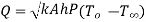
Heat transfer at base is equal to heat transfer through fin. Hence, at base(x=0)

From 1.21
As x=0
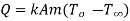


…(1.23)
2. Adequately long fin with insulated fin
Boundary conditions are
At  hence
hence  .
.
At 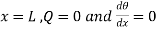
Applying first boundary condition on 1.18

…(1.24)
Fig 1.16 Insulated fin
Applying second boundary condition on 1.19

…(1.25)
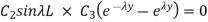
From 1.25

Substituting C1 and C2 in 1.18
But 
…(1.26)
This represents temperature distribution on insulated long fin.
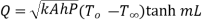
Heat transfer at base is equal to heat transfer through fin. Hence, at base(x=0)

From 1.26
Therefore at x=0
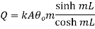

…(1.27)
3. Short Fin

Fig.1.17 Short fin
Boundary conditions are
At  hence
hence 
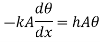
At 
 is heat convected away to surrounding.
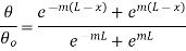
From second boundary condition at x=L,
From 1.18 and 1.19


…(1.28)
Putting boundry condition 1 in 1.18

Solving this equation and 1.28
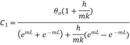
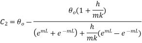
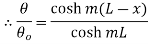
Putting these values in 1.18
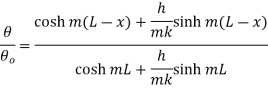
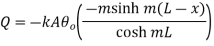
At x=L and 
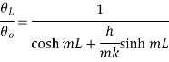
This represents temperature distribution on short fin.
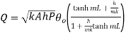
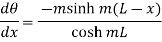
 at x=0
Substituting 
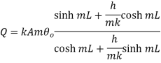

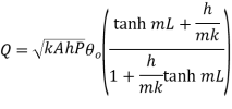
…(1.29)
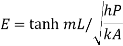
1.7.2. Effectiveness of fin
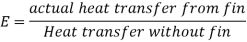


For infinitely long fin tanhmL=1


1.8.1. Lumped system approximation
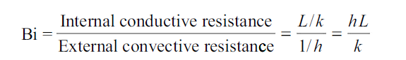
where h is the average heat transfer coefficient, L is a characteristic dimension obtained by dividing the volume of the body by its surface area and k is the thermal conductivity of the solid body. For Bi < 0.1, i.e. when the internal resistance is less than 10% of the external resistance, the internal resistance can be ignored and lumped system approximation can be used.
1.8.2 Heisler charts
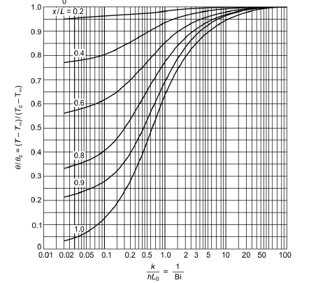
Fig 1.18 Temperature as a function of centre temperature in an infinite plate of thickness 2L
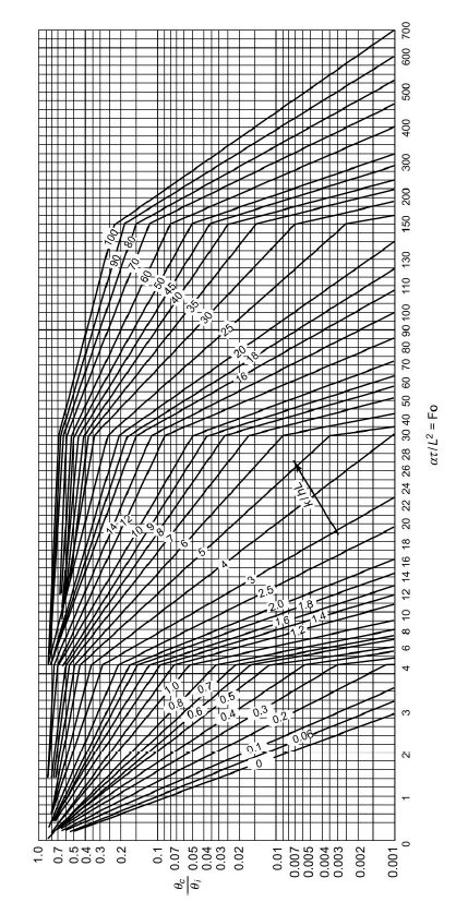
Fig 1.19 Axis temperature for infinite plate with thickness 2L
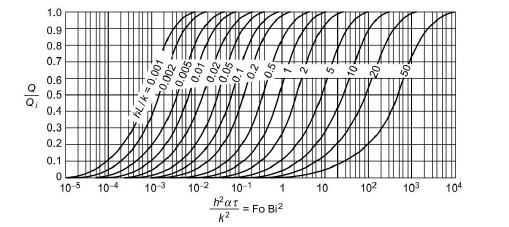
Fig 1.20 Heat loss of an infinite plate of thickness 2L with time
These are Heisler charts for cylinder where,
Fo = Fourier number
Bi=Biot number
 =Thermal diffusivity
h= convective heat transfer coefficient
Q=Heat transfer rate
Qi=Heat transfer rate at t=0
t=time
When the boundaries of a system are irregular or the temperature along a boundary is non-uniform, a one-dimensional treatment may not be satisfactory. Temperature here may be a function of two or even three coordinates.
The components of the heat flow per unit area (heat flux) q in the x and y-direction are obtained from Fourier’s law:
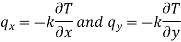
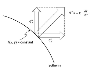
Fig.1.21 Heat flow in two dimensions
The heat flux q at a given point (x, y) is the resultant of the components qx and qy at that point and is directed perpendicular to the isotherm (Fig.1.21). If the temperature distribution in a system is known, the rate of heat flow can easily be calculated.
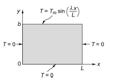
Fig.1.22 Rectangular adiabatic plate with sinusoidal temperature distribution on one edge
Let us consider a simple case of a thin rectangular plate (Fig. 1.22), free of heat sources and insulated at the top and bottom surfaces. Since ∂T/∂z =0, the temperature is a function of x and y only. If k is uniform, the temperature distribution must satisfy Eq. (2.134), a linear and homogeneous partial differential equation that can be integrated by assuming a product solution for T(x, y) of the form

…(1.30)
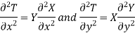
where X = X(x), a function of x only, and Y = Y(y), a function of y alone. Differentiating above equation twice, first with respect to x and then with respect to y.
Substituting this values in 1.30
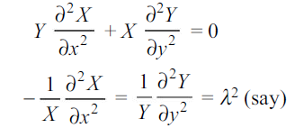
The variables are now separated. The LHS is a function of x only, while the RHS is a function of y alone. Since neither side can change as x and y vary, both must be equal to a constant, say  . We have, therefore, two ordinary differential equations

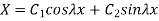
Solutions to above differential equations are
And

respectively. Substituting these values in 1.30

…(1.31)
where C1, C2, C3 and C4 are constants to be evaluated from the boundary conditions. As shown in Fig. 1.22, the boundary conditions to be satisfied are
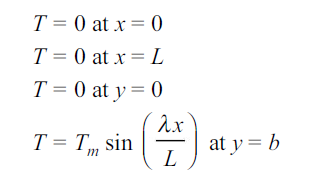
Substituting third condition in 1.31

…(1.32)
Substituting first condition in 1.31
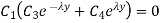
…(1.33)
Substituting second condition in 1.31

…(1.34)
Solving 1.33,  , solving 1.32, we get
Using these results in 1.34
To satisfy this condition, sin  L = 0 or,
  =
= , where n = 1, 2, 3, …. There exists, therefore, a different solution for each integer n, and each solution has a separate integration constant Cn. Summing these solutions
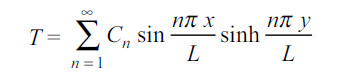
…(1.35)

Putting this value in 1.35
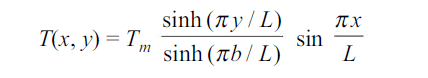
…(1.36)
For regular shaped bodies, analytical methods in the form of Heisler’s charts can be used to determine the time-temperature history.
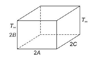
Fig. 1.23 A parallelepiped being heated or cooled
Let us consider a rectangular parallelepiped with dimensions 2A, 2B and 2C, which is initially at a uniform temperature Ti and then subjected to a constant surrounding temperature  (Fig.1.23).
Fourier’s heat conduction equation in absence of any heat source is given by
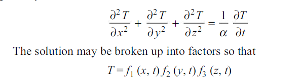
Substituting above mentioned factors in fourier equation
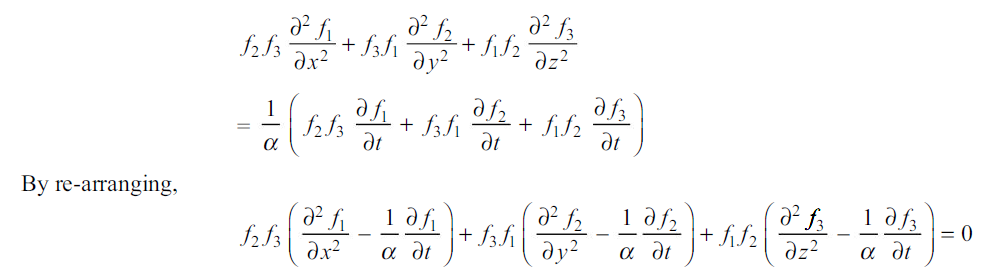
…(1.37)
Equation 1.37 will be satisfied only if
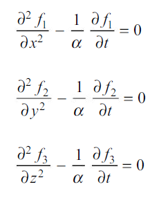
But these are simply three one-dimensional forms of Fourier’s equation, so that the solution to the three-dimensional problem may be expressed as the product of three solutions of one-dimensional problems.
From Heisler’s charts for infinite plates, ( /
/ )A, (
)A, ( /
/ ))B and (
 /
/ ))C are found out. The product of these three will give the centre temperature of the parallelepiped

Conductive heat transfer |
|
Convective heat transfer |
|
Radiation heat transfer |
|
Heat balance equation |
|
Conductive thermal resistance |
|
Convective thermal resistance |
|
Total thermal resistance of bodies connected in series |
|
Total thermal resistance of bodies connected in parallel |
|
Heat transfer through cylinder |
|
Heat transfer through sphere |
|
Critical insulation radius of cylinder |
|
Critical insulation radius of sphere |
|
Heat transfer through infinitely long fin |
|
Heat transfer through fin with insulated tip |
|
Heat transfer through short fin |
or
|
Effectiveness of fin |
|
Biot number |
|