UNIT 8
Digital filter structure
FIR DESIGN
Design of linear phase FIR filter using windows and frequency sampling method
The frequency sampling method is use to design recursive and non-recursive FIR filters for both standard frequency selective filters and with arbitrary frequency response. The main idea of the frequency sampling design method is that a desired frequency response can be approximated by sampling it at N evenly spaced points and then obtaining N-point filter response.
A continuous frequency response is then calculated as an interpolation of the sampled frequency response. The approximation error would then be exactly zero at the sampling frequencies and would be finite in frequencies between them. The smoother the frequency response being approximated, the smaller will be the error of interpolation between the sample points.
There are two distinct types of Non-Recursive Frequency Sampling method of FIR filter design, depending on where the initial frequency sample occurred. The type 1 designs have the initial point at ω=0, whereas the type 2 designs have the initial point at f=1/2N or ω=π/N.
Procedure for Type I design
- Choose the desired frequency response

- Samples
 at N points by taking
  where
where 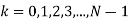 generate the sequence H (k). To obtain a good approximation of the desired frequency response, a sufficiently large number of the frequency samples should be taken
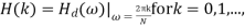
- The N point inverse DFT of the sequence H (k) gives the impulse response of the filter h (n). For a practical realization of the filter, samples of impulse response should be real. This can happen if all the complex terms appears in conjugate pairs.
Desired filter coefficients
For linear phase filter with positive symmetrical impulse response,
4) Take z transform of the impulse response h (n) to get the filter transfer function H (z)
Procedure for Type 2 Design
(Same steps as above expect step 2)
2) Samples  at N points by taking
  where
where  generate the sequence H (z)

Type 2 frequency samples gives additional flexibility in the design method to satisfy the desired frequency response at a second possible set of frequencies.
Frequency response of linear phase FIR filters
“Linear Phase” refers to the condition where the phase response of the filter is a linear (straight-line) function of frequency (excluding phase wraps at +/- 180 degrees). This results in the delay through the filter being the same at all frequencies. Therefore, the filter does not cause “phase distortion” or “delay distortion”. The lack of phase/delay distortion can be a critical advantage of FIR filters over IIR and analog filters in certain systems, for example, in digital data modems.
For an N-tap FIR filter with coefficients h (k), whose output is described by:
y(n)=h(0)x(n) + h(1)x(n-1) + h(2)x(n-2) + … h(N-1)x(n-N-1), the filter’s Z transform is:
H(z)=h(0)z-0 + h(1)z-1 + h(2)z-2 + … h(N-1)z-(N-1) , or
The variable z in H (z) is a continuous complex variable, and we can describe it as: z=r·ejw, where r is a magnitude and w is the angle of z. If we let r=1, then H (z) around the unit circle becomes the filter’s frequency response H (jw). This means that substituting ejw for z in H (z) gives us an expression for the filter’s frequency response H (w), which is:
H(jw)=h(0)e-j0w + h(1)e-j1w + h(2)e-j2w + … h(N-1)e-j(N-1)w , or
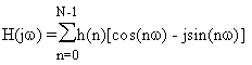
Using Euler’s identity, e-ja=cos (a) – jsin (a), we can write H (w) in rectangular form as:
H (jw)=h(0)[cos (0w) – jsin (0w)] + h(1)[cos (1w) – jsin (1w)] + … h (N-1)[cos ((N-1)w) – jsin ((N-1)w)] , or
FIR filters realization using direct form, cascade form
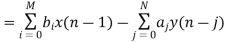
The direct form is obtained from
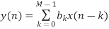
Based on the above equation, we need the current input sample and M−1 previous samples of the input to produce an output point. For M=5, we can simply obtain the following diagram from Equation 1.
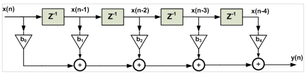
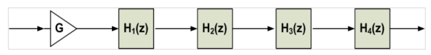
On the other hand, for a linear-phase FIR filter, we observe the following symmetry in coefficients of the difference equation
The structure obtained from the above equation is shown in Figure 2. While Figure 1 requires five multipliers, employing the symmetry of a linear-phase FIR filter, we can implement the filter using only three multipliers. This example shows that for an odd M, the symmetry property reduces the number of multipliers of an (M−1)th-order FIR filter from M to M+1/2.
Cascade form
The cascade structure is obtained from the system function H(z). The idea is to decompose the target system function into a cascade of second-order FIR systems. In other words, we need to find second-order systems which satisfy
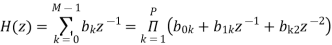
Where P is the integer part of M/2. For example, M=5, H(z) will be a polynomial of degree four which can be decomposed into two second-order sections. Each of these second-order filters can be realized using a direct form structure. It is desirable to set a pair of complex-conjugate roots for each of the second-order sections so that the coefficients become real.
Assume that we need to implement the nine-tap FIR filter given by the following table using a cascade structure.
k | 4 | 3 and 5 | 2 and 6 | 1 and 7 | 0 and 8 |
 | 0.3333 | 0.2813 | 0.1497 | 0 | -0.0977 |
Solution:
The system function of this filter is

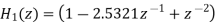
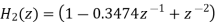
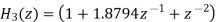
It can be show
Where

IIR DESIGN
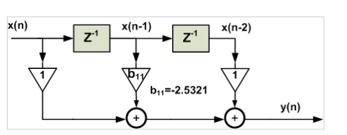
Concept of analog filter design
Filters are networks that process signals in a frequency-dependent manner. The basic concept of a filter can be explained by examining the frequency dependent nature of the impedance of capacitors and inductors. Consider a voltage divider where the shunt leg is a reactive impedance.
As the frequency is changed, the value of the reactive impedance changes, and the voltage divider ratio changes. This mechanism yields the frequency dependent change in the input/output transfer function that is defined as the frequency response.
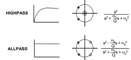
A simple, single-pole, high-pass filter can be used to block dc offset in high gain amplifiers or single supply circuits. Filters can be used to separate signals, passing those of interest, and attenuating the unwanted frequencies.
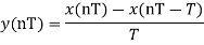
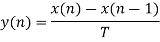
IIR filter design by approximation of derivatives
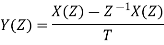
Consider an analog filter. Its transfer function will be of the differential equation form as shown below.

Taking Laplace transform on both ends:

The transfer function of the analog filter can be given by:
Note that this is just a generic transfer function. To get the transfer function of a digital filter we will dive into some specifics.
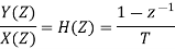
Thus,
Taking z-transform on both sides:
Solving for the transfer function of the digital filter:
The mapping between S and Z planes
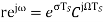
To map from s to z-plane we need to find the values of σ and Ω in s = σ + jΩ. We have the relationship between s and z from above as:

Rewriting the above equation for z:

Substituting s = σ+jΩ in the above equation and solving gives us:
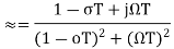
Separating the real and imaginary parts we get:
For σ=0
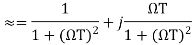
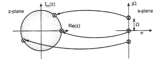
When we vary Ω from -∞ to +∞, the corresponding locus of points in the z-plane is a circle with radius 1/2 and with its centre at z=1/2.
Similarly, when we map the equation  the left half-plane of the s-domain maps inside the circle with 0.5 radians. Moreover, the right half-plane of the s-domain is mapped outside the unit circle.
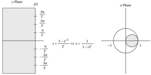
Mapping of s-plane into the z-plane by the approximation of derivatives method.
Thus we can say that this transformation of an analog filter results in a stable digital filter.
Limitations:
From the above fig, the location of poles in the z-domain is confined to smaller frequencies. Thus the approximation of derivatives method is limited to designing low pass and band pass IIR filters with small resonant frequencies only. It can’t be used to develop high pass and band-reject filters.
IIR filter design by impulse invariance method
The Impulse Invariance Method is used to design a discrete filter that yields a similar frequency response to that of an analog filter. Discrete filters are amazing for two very significant reasons:
- You can separate signals that have been fused and,
- You can use them to retrieve signals that have been distorted.
We can design this filter by finding out one very important piece of information i.e., the impulse response of the analog filter. By sampling the response we will get the time-domain impulse response of the discrete filter.
When observing the impulse responses of the continuous and discrete responses, it is hard to miss that they correspond with each other. The analog filter can be represented by a transfer function, Hc(s).
Zeros are the roots of the numerator and poles are the roots of the denominator.
Mapping from s-plane to z-plane
The transfer function of the analog filter in terms of partial fraction expansion with real coefficients is
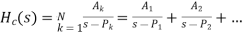 Where A are the real coefficients and P, are the poles of the function And k can be 1, 2 …N.
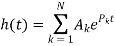
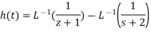
h (t) is the impulse response of the same analog filter but in the time domain. Since, ‘s’ represents a Laplace function Hc (s) can be converted to h(t), by taking its inverse Laplace transform.
Using this transformation,
We obtain
However, in order to obtain a discrete frequency response, we need to sample this equation. Replace ‘nTS’ in the place of t where TS represents the sampling time. This gives us the sampled response h(n),
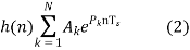
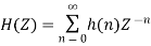
Now, to obtain the transfer function of the IIR Digital Filter which is of the ‘z’ operator, we have to perform z-transform with the newly found sampled impulse response, h (n). For a causal system which depends on past (-n) and current inputs (n), we can get H (z) with the formula shown below
We have already obtained the equation for h (n). Hence, substitute eqn. (2) into the above equation
Factoring the coefficient and the common power of n
— (3)
Based on the standard summation formula, (3) is modified and written as the required transfer function of the IIR filter.
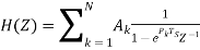 – (4)
– (4)
Hence (4) is obtained from (1), by mapping the poles of the analog filter to that of the digital filter.
That is how you map from the s-plane to z-plane
Relationship of S-plane to Z plane
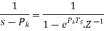
From the equation above, Since, the poles are the denominators we can say,  .
.
Comparing (1) and (4), we can derive that
 – (5)
– (5)
And since  , substituting into (5) gives us
 –(6)
–(6)
Where
TS is the sampling time
Now, s is taken to be the Laplace operator
 – (7)
– (7)
σ is the attenuation factor
Ω is the analog frequency
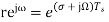
Changing Z from rectangular coordinates to the polar coordinates, we get:
 – (8)
– (8)
Where r is magnitude and ω is digital frequency
Replacing (7) in place of s, in (6), and replacing that value as Z in (8)
Compare the real and imaginary parts separately. Where the component with ‘j’ is imaginary.
 –(9)
–(9)
And

Hence, we can make the inference that

To understand the relationship between the s-plane and Z-plane, we need to picture how they will be plotted on a graph. If we were to plot (7) in the ‘s’ domain, σ would be the X-coordinates and jΩ would be the Y-coordinate. Now, if we were to plot (8) in the ‘Z’ domain, the real portion would be the X-coordinate, and the imaginary part would be the Y-coordinate.
Let us take a closer look at equation (9),

There are a few conditions that could help us identify where it is going to be mapped on the s-plane.
Case 1
When σ <0, it would translate that r is the reciprocal of ‘e’ raised to a constant. This will limit the range of r from 0 to 1.
Since σ <0, it would be a negative value and would be mapped on the left-hand side of the graph in the ‘s’ domain
Since 0<r<1, this would fall within the unit circle which has a radius of in the ‘z’ domain.
Case 2
When σ =0, this would make r=e0, which gives us 1, which means r=1. When the radius is 1, it is a unit circle.
Since σ =0, which indicates the Y-axis of the ‘s’ domain.
Since r=1, the point would be on the unit circle in the ‘z’ domain.
Case 3
When σ>0, since it is positive, r would be equal to ‘e’ raised to a particular constant, which means r would also be a positive value greater than 1.
Since σ>0, the positive value would be mapped onto the right-hand side of the ‘s’ domain.
Since r>1, the point would be mapped outside the unit circle in the ‘z’ domain.
Here is a pictorial representation of the three cases:
Mapping of poles located at the imaginary axis of the s-plane onto the unit circle of the z-plane. This is an important condition for accurate transformation.
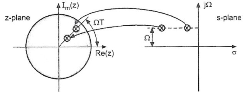
Mapping of the stable poles on the left-hand side of the imaginary s-plane axis into the unit circle on the z-plane. Poles on the right-hand side of the imaginary axis of the s-plane lie outside the unit circle of the z-plane when mapped.
Disadvantages:
- Digital frequency represented by ‘ω,’ and its range lies between – π and π. Analog frequency is represented by ‘Ω,’ and its range lies between – π/TS and π/TS. When mapping from digital to analog, from – π/TS and π/TS , ‘ω’ maps from – π to π. This would make the range of Ω (k-1) π/TS and (k+1) π/TS, where k is an arbitrary constant. However, mapping the other way, from analog to digital, will mean ω maps from – π to π, which makes it many-to-one. Hence, mapping is not one-to-one.
- Analog filters do not have a definite bandwidth because of which when sampling is performed, this would give rise to aliasing. Aliasing is when the signal eats up into the next signal and so on. This would lead to considerable distortion of the signal. Hence, making the frequency response of the converted digital signal very different from the original frequency response of the analog filter.
- Increasing the sampling time will result in a frequency response that is more spaces out hence decreasing the chances of aliasing. However, this is not the case with this method. Increasing the sampling time has no effect on the amount of aliasing that happens.
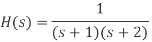
Given, 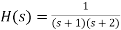 , that has a sampling frequency of 5Hz. Find the transfer function of the IIR digital filter.
Solution:
Step 1:
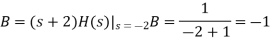
Step 2:
Applying partial fractions on H(s),

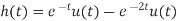
Step 3:
Step 4:
IIR filter realization using direct form
Direct form I
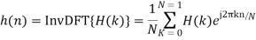
The difference equation,


Specifies the Direct-Form I (DF-I) implementation of a digital filter. The DF-I signal flow graph for the second-order case is shown in Fig.
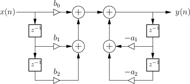 |
Figure: Direct-Form-I implementation of a 2nd-order digital filter. |
Direct form II
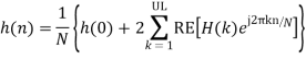
The signal flow graph for the Direct-Form-II (DF-II) realization of the second-order IIR filter section is shown in Fig.
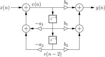 |
Figure: Direct-Form-II implementation of a 2nd-order digital filter. |
The difference equation for the second-order DF-II structure can be written as


Which can be interpreted as a two-pole filter followed in series by a two-zero filter.
Finite word length effect in IIR filter design
Digital Signal Processing the computations like FFT algorithm, ADC and filter designs are associated with numbers and coefficients.
• These numbers and coefficients are stored in a finite length registers but due to mathematical manipulations perform with fixed point arithmetic number of errors are present by storing the numbers and coefficients are required to quantize the different type of number representations are used for this purpose.
• The implementation of digital filters involves the use of finite precision arithmetic. This leads to quantization of the filter coefficients and the results of the arithmetic operations. Such quantization operations are nonlinear and cause a filter response substantially different from the response of the underlying infinite-precision model.
• Finite word length of the signals to be processed the finite word length of the filter coefficients does not affect the linearity of the filter behaviour. This effect only amounts to restrictions on the linear filter characteristics, resulting in discrete grids of pole-zero patterns.
• These effects, which divide into those due to "signal quantization" and those due to "overflow".


