Unit-4
Design of Digital filters
In practice it may be impossible to use all the terms of a Fourier series. For example, suppose we have a device that manipulates a periodic signal by first finding the Fourier series of the signal, then manipulating the sinusoidal components, and, finally, reconstructing the signal by adding up the modified Fourier series. Such a device will only be able to use a finite number of terms of the series.
Gibbs’ phenomenon occurs near a jump discontinuity in the signal. It says that no matter how many terms you include in your Fourier series there will always be an error in the form of an overshoot near the discontinuity.
The overshoot always be about 9% of the size of the jump. We illustrate with the example. Of the square wave sq(t). The Fourier series of sq(t) fits it well at points of continuity. But there is always an overshoot of about .18 (9% of the jump of 2) near the points of discontinuity.
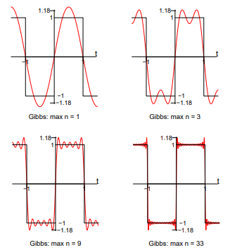
Fig 1 Gibbs Phenomenon
In these figures, for example, ’max n=9’ means we included the terms for n = 1, 3, 5, 7 and 9 in the Fourier sum
Windowing method
Let the frequency response of the desired LTI ststem we wish to approximate be given by
Where  is the corresponding impulse response.
Consider obtaining a casual FIR filter that approximates  by letting
The FIR filter then has frequency response
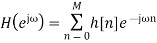
Note that sibce we can write
We are actually forming a finite Fourier series approximation to 
Since the ideal  may contain discontinuities at the band edges, truncation of the Fourier series will result in the Gibbs phenomenon.
To allow for a less abrupt Fourier series truncation and hence reduce Gibbs phenomenon oscillations, we may generalize h [n] by writing
Where  is a finite duration window function of length M +1.
Park-McClellan's method
The Parks–McClellan algorithm, published by James McClellan and Thomas Parks in 1972, is an iterative algorithm for finding the optimal Chebyshev finite impulse response filter. The Parks–McClellan algorithm is utilized to design and implement efficient and optimal FIR filters. It uses an indirect method for finding the optimal filter coefficients.
The Parks–McClellan Algorithm is implemented using the following steps:
- Initialization: Choose an extremal set of frequences {ωi(0)}.
- Finite Set Approximation: Calculate the best Chebyshev approximation on the present extremal set, giving a value δ(m) for the min-max error on the present extremal set.
- Interpolation: Calculate the error function E(ω) over the entire set of frequencies Ω using (2).
- Look for local maxima of |E(m)(ω)| on the set Ω.
- If max(ωεΩ)|E(m)(ω)| > δ(m), then update the extremal set to {ωi(m+1)} by picking new frequencies where |E(m)(ω)| has its local maxima. Make sure that the error alternates on the ordered set of frequencies as described in (4) and (5). Return to Step 2 and iterate.
- If max(ωεΩ)|E(m)(ω)| ≤ δ(m), then the algorithm is complete. Use the set {ωi(0)} and the interpolation formula to compute an inverse discrete Fourier transform to obtain the filter coefficients.
The Parks–McClellan Algorithm may be restated as the following steps:
- Make an initial guess of the L+2 extremal frequencies.
- Compute δ using the equation given.
- Using Lagrange Interpolation, we compute the dense set of samples of A(ω) over the passband and stopband.
- Determine the new L+2 largest extrema.
- If the alternation theorem is not satisfied, then we go back to (2) and iterate until the alternation theorem is satisfied.
- If the alternation theorem is satisfied, then we compute h(n) and we are done.
To gain a basic understanding of the Parks–McClellan Algorithm mentioned above, we can rewrite the algorithm above in a simpler form as:
- Guess the positions of the extrema are evenly spaced in the pass and stop band.
- Perform polynomial interpolation and re-estimate positions of the local extrema.
- Move extrema to new positions and iterate until the extrema stop shifting.
Key takeaway
The windowing technique is simple and has minimum computation. The maximum ripple amplitude in filter response is fixed regardless of how large the filter order is.
Butterworth filter design
At the expense of steepness in transition medium from pass band to stop band this Butterworth filter will provide a flat response in the output signal. So, it is also referred as a maximally flat magnitude filter. The rate of falloff response of the filter is determined by the number of poles taken in the circuit. The pole number will depend on the number of the reactive elements in the circuit that is the number of inductors or capacitors used in the circuits.
The amplitude response of nth order Butterworth filter is given as follows:
Vout / Vin = 1 / √{1 + (f / fc)2n}
Where ‘n’ is the number of poles in the circuit. As the value of the ‘n’ increases the flatness of the filter response also increases.
'f' = operating frequency of the circuit and 'fc' = centre frequency or cut off frequency of the circuit.
These filters have pre-determined considerations whose applications are mainly at active RC circuits at higher frequencies. Even though it does not provide the sharp cut-off response it is often considered as the all-round filter which is used in many applications.
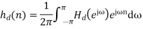
First Order Low Pass Butterworth Filter
The below circuit shows the low pass Butterworth filter:
Fig 2 First order LP Butterworth Filter
The required pass band gain of the Butterworth filter will mainly depends on the resistor values of ‘R1’ and ‘Rf’ and the cut off frequency of the filter will depend on R and C elements in the above circuit.
The gain of the filter is given as Amax = 1 + (R1 / Rf)
The impedance of the capacitor ‘C’ is given by the -jXC and the voltage across the capacitor is given as,
Vc = - jXC / (R - jXC) * Vin
Where XC = 1 / (2πfc), capacitive Reactance.
The transfer function of the filter in polar form is given as
H(jω) = |Vout/Vin| ∟ø
Where gain of the filter Vout / Vin = Amax / √{1 + (f/fH)²}
And phase angle Ø = - tan-1 ( f/fH )
At lower frequencies means when the operating frequency is lower than the cut-off frequency, the pass band gain is equal to maximum gain.
Vout / Vin = Amax i.e. constant.
At higher frequencies means when the operating frequency is higher than the cut-off frequency, then the gain is less than the maximum gain.
Vout / Vin < Amax
When operating frequency is equal to the cut-off frequency the transfer function is equal to Amax /√2. The rate of decrease in the gain is 20dB/decade or 6dB/octave and can be represented in the response slope as -20dB/decade.
Second Order Low Pass Butterworth Filter
An additional RC network connected to the first order Butterworth filter gives us a second order low pass filter. This second order low pass filter has an advantage that the gain rolls-off very fast after the cut-off frequency, in the stop band.
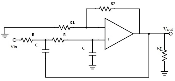
Fig 3 Second Order LP Butterworth Filter
In this second order filter, the cut-off frequency value depends on the resistor and capacitor values of two RC sections. The cut-off frequency is calculated using the below formula.
fc = 1 / (2π√R2C2)
The gain rolls off at a rate of 40dB/decade and this response is shown in slope -40dB/decade. The transfer function of the filter can be given as:
Vout / Vin = Amax / √{1 + (f/fc)4}
The standard form of transfer function of the second order filter is given as
Vout / Vin = Amax /s2 + 2εωns + ωn2
Where ωn = natural frequency of oscillations = 1/R2C2
ε = Damping factor = (3 - Amax ) / 2
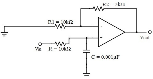
For second order Butterworth filter, the middle term required is sqrt(2) = 1.414, from the normalized Butterworth polynomial is
3 - Amax = √2 = 1.414
In order to have secured output filter response, it is necessary that the gain Amax is 1.586.
Higher order Butterworth filters are obtained by cascading first and second order Butterworth filters.
n (order)
Normalized Denominator polynomials in factored form
1

2
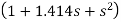
3
The transfer function of the nth order Butterworth filter is given as follows:
H(jω) = 1/√{1 + ε² (ω/ωc)2n}
Where n is the order of the filter
ω is the radian frequency and it is equal to 2πf
And ε is the maximum pass band gain, Amax
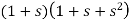
Examples
Let us consider the Butterworth low pass filter with cut-off frequency 15.9 kHz and with the pass band gain 1.5 and capacitor C = 0.001µF.
fc = 1/2πRC
15.9 * 10³ = 1 / {2πR1 * 0.001 * 10-6}
R = 10kΩ
Amax = 1.5 and assume R1 as 10 kΩ
Amax = 1 + {Rf / R1}
Rf = 5 kΩ
Ideal Frequency Response of the Butterworth Filter
The flatness of the output response increases as the order of the filter increases. The gain and normalized response of the Butterworth filter for different orders are given below:
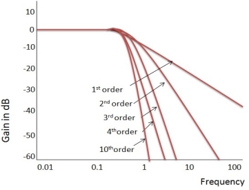
Fig 4 Frequency Response of Butterworth Filter
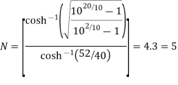
Example. A Butterworth Amplitude Response design
Let, 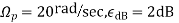
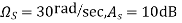
Solving for N gives
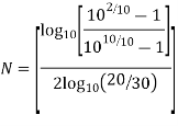
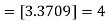
Matching at 
The normal  from the table is
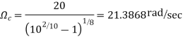
Frequency seal 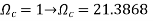 impliea that we let
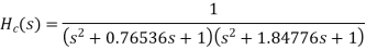
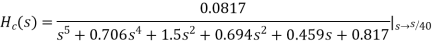
Finally, the frequency scaled system function is
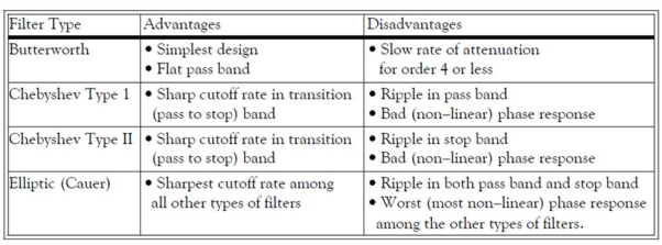
Chebyshev filters and elliptic filters
A Chebyshev design achieves a more rapid roll-off rate near the cut-off frequency than the Butterworth by allowing ripple in the passband (type I) or stopband (type II). Monotonicity of the stopband or passband is still maintained respectively.
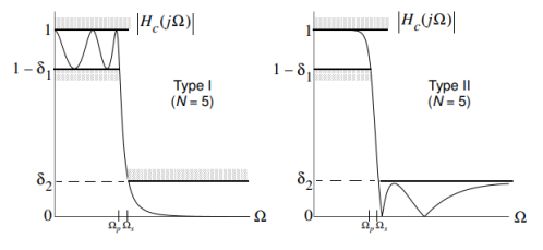
Fig 5 Chebyshev Filter Type I and II
Chebyshev Type I
The magnitude response is given by
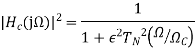
Where,
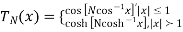
 Nth order Chebyshev polynomial
And  specifies the passband ripple
The Chebyshev polynomials are of the form\

With recurrence formula

An alternate form for  which will be useful in both analysis and design is
Design a Chebyshev type I lowpass filter to satisfy the following amplitude specification 
Using the design formula for N
From the 2dB ripple table (9-20)
Elliptic Design
Allows both passband and stopband ripple to obtain a narrow transition band. The elliptic (Cauer) filter is optimum in the sense that no other filter of the same order can provide a narrower transition band.
The squared magnitude response is given by
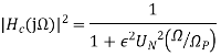
Fig 6 Magnitude Response
Define the transition region ratio as

The normalized lowpass system function can be written in factored form as
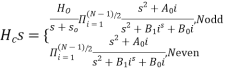
Note:  contains conjugate pairs of zeros on the j
 axis which give the stopband nulls.
The filter coefficients  if N is odd.
Design an elliptic lowpass filter to satisfy the following amplitude specifications, 
From the 1dB ripple, 40Db stopband attenuation table wew find that N meets or exceeds the
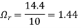
  = 1.2187, so we can scale
 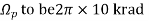 and then the desired stopband attenuation will actually be achieved at
  .
.
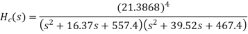
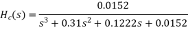
T6he normalized H (z)  is
is
H(s)=(0.046998s4+0.22007s2+0.22985)/(s5+0.92339s4+1.84712s3+1.12923s2+0.78813s
To complete the design scale H (s) by letting 
Example. Design from a Rational H (s)
Let, 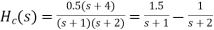
Inverse Laplace transforming yields
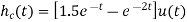
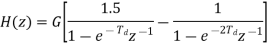
Sampling  seconds and gain scaling we obtain

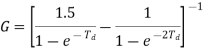
Which implies that
Setting  requires that
Design a Chebyshev type 1 low pass filter to satisfy the following amplitude specifications: 
Using the design formula for N
N = [2.08]=3
Note: 
The normalized system function is
With poles at
To frequency scale  let
let
So in the z domain
Note that when the design originates from discrete time specifications the poles of H (z) are independent of  .
.
Design of Low-pass, Band-pass, Band-stop and High-pass filters.
The procedure to design high-pass, band-pass or band-stop digital filter is listed in the following steps.
- Write the digital filter specifications.
- From these specifications find the normalized low-pass filter H(s).
- For LPF and HPF have only one critical frequency but for BPF and BSF we have lower and upper band edge frequencies ω1 and ω2.
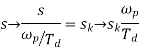
- Replace the S in transfer function H(s)
S=s/ ωp From LPF to LPF
S= ωp/s From LPF to HPF
S=  From LPF to BPF
S= From LPF to BSF
 = ω1 ω2
W = ω2- ω1
- Find Lower edge frequency and Upper band edge frequency
Example
Design a digital filter for given specifications cut-off frequency =30Hz, sampling frequency=150Hz. The filter should be HPF.
Sol: First order transfer function of LPF is
Step 1: HL(s) = 
Step 2: Prewrap critical frequency
Ωp = tan(ωp Ts/2)= tan[(30x2xπ)/(2x150)] =0.7265
Step 3: Using LPF to HPF Transformation equation
HH(s) = HL(s) =  =
=  =
= 
For LPF
H(z) = HH(s) for s= 
HH(s) = = 0.5792 [
  ]
]
Design a BPF with pass band of 200-300 Hz, sampling frequency 2000Hz and filter order 2.
Sol:
STEP 1: Passband edge frequency ω1 =200Hz
ω2= 300Hz
STEP 2: Prewrap critical frequency
Ω1 = tan(ω1 Ts/2)= tan(200xπ/2000) = 0.3249
Ω2 = tan(ω2 Ts/2)= tan(300xπ/2000) = 0.5095
STEP 3:  = Ω1 Ω2 = 0.3249 x 0.5095 = 0.1655
W = Ω2 – Ω1 = 0.5095-0.3249 = 0.1846
STEP 4:HB(s) = HL(s) for s = S= 
For LPF
H(z) = 
HB(s) =  =
=  =
= 
STEP 5: Replace s by 
HB(s) =
H(z) = 0.1367 [ 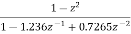 ]
]
Key takeaway
Digital Signal Processing the computations like FFT algorithm, ADC and filter designs are associated with numbers and coefficients.
• These numbers and coefficients are stored in a finite length registers but due to mathematical manipulations perform with fixed point arithmetic number of errors are present by storing the numbers and coefficients are required to quantize the different type of number representations are used for this purpose.
• The implementation of digital filters involves the use of finite precision arithmetic. This leads to quantization of the filter coefficients and the results of the arithmetic operations. Such quantization operations are nonlinear and cause a filter response substantially different from the response of the underlying infinite-precision model.
• Finite word length of the signals to be processed the finite word length of the filter coefficients does not affect the linearity of the filter behaviour. This effect only amounts to restrictions on the linear filter characteristics, resulting in discrete grids of pole-zero patterns.
• These effects, which divide into those due to "signal quantization" and those due to "overflow".
Parametric spectral estimation
Parametric or Model-based methods find an ARMA type model for the data, then estimate the parameters of the model, and then substitute the estimates of the parameters into the formula for the true f, thus giving an estimate of f. However, these methods require the availability of long data records in order to obtain the necessary frequency resolution required in many applications. Furthermore, these methods suffer from spectral leakage effects, due to windowing.
In fact, these methods extrapolate the values of the autocorrelation for lags m > N. Extrapolation is possible if we have some a priori information on how the data were generated. In such a case a model for the signal generation can be constructed with a number of parameters that can be estimated from the o b served data. From the model and the estimated parameters, we can compute the power density spectrum im plied by the model. In effect, the modeling approach eliminates the need for window functions and the assumption that the auto correlation sequence is zero for |m| > N.
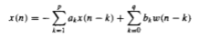
As a consequence, parametric (model-based) pow er spectrum estimation methods avoid the problem of leakage and provide better frequency resolution than do the FFT - based, non -parametric methods described in the preceding section. This is especially true in applications where short data records are available due to time-variant or transient phenomena. The parametric methods considered in this section are based on modeling the data sequence x(n) as the output of a linear system characterized by a rational system function of the form
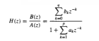
The difference equation is given by
Non-parametric spectral estimation
Nonparametric or Non-Model based methods smooth the sample spectral density  without making any assumption about a model for the data.
Weighted Averages of 
If we want to estimate f at one of the natural frequencies ωk, a natural thing to do would be to use  M(ωk) = the average of
  (ωk) and the M values of
  on either side of
  (ωK). This would give
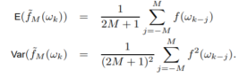
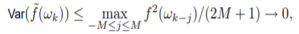
In any frequency band where f is not changing much, the expectation will be approximately f, while for places where f is changing, a bias will be introduced. Note that
Just doing straight moving averages is not the most efficient way to do the averaging. We need to do weighted averages
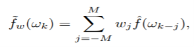
Where the weight applied to  (ωj ) for ωj close to ωk is larger than for one far away from ωk. (Note that we want to use symmetric weights, that is, w−j = wj , since we want equal weight applied to
  ’s equally distant from the “target frequency” ωk.).
A useful way to determine a set of weights w0,...,wM is to “sample” a continuous function that looks like a weight function (high in the middle, falls off on either side of the middle) λ(x), where λ(x) is defined only on the interval [−1, 1]. Thus, we let
wj = λ(j/M), j = 0, 1,...,M.
The table below gives eight standard weight functions (the first five are zero outside [−1, 1] while the others are not).
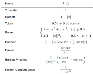
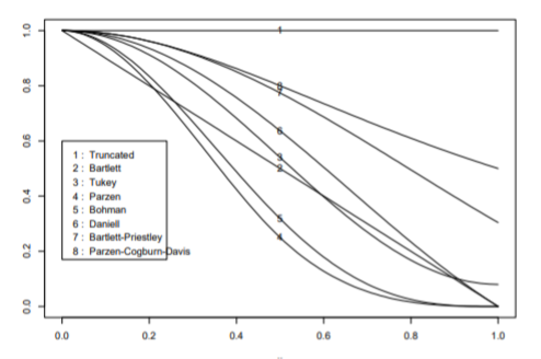
Fig 7 Eight weight Functions [Ref6]
Applying Kernels to Sample Autocovariances
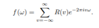
Another way to smooth the periodogram is to notice that the sample spectral density can be written as
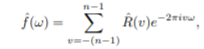
Which is estimating the true spectral density function
Thus there are two problems with  :
:
1. Truncation error: Truncating the sum at −(n − 1) to (n − 1).
2. Estimation error: Having to use the estimator  (v) for R(v).
A great deal of study has been done on “speeding up” the convergence of Fourier series by applying weights to the  (v)’s which would give a new spectral estimator:
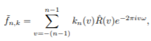
If we sample the same weight functions we looked before, that is, use kn(v) = λ(v/M), then we get
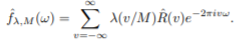
This estimator can also be viewed as smoothing ˆf as a little algebra shows
Thus  λ,M(ω) is an integrated weighted average of
  .
.
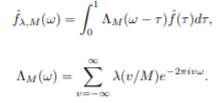
Key takeaway
The function λ is called a lag window generator, the function kn(v) = λ(v/M) is called a lag window, and the function ΛM is called a spectral window. If λ(x)=0 outside of [−1, 1], then
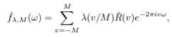
And the “scale parameter” M is called a truncation point.
The process of sampling rate conversion in the digital domain can be view ed as a linear filtering operation, as illustrated in Fig below. The input signal x(n) is characterized by the sampling rate Fx = 1/Tx and the output signal y(m) is characterized by the sampling rate Fv = 1/Ty, where Tx an d Ty are the corresponding sampling intervals. In the m ain p a rt of our treatment, the ratio Fy/Fx is constrained to be rational,
Fy/Fx =I/D
w here D and I are relatively prim e integers. We shall show that the linear filter is characterized by a time-variant im pulse response, denoted as h(n,m). Hence the input x(n) and the output v(m) are related by the co n volution summation for time-variant systems.
The sampling rate conversion can be determined by the digital resampling of the same analog signal. If x(t) is the analog signal that is sampled at the first rate Fx so that we obtain x(n). The main aim is to directly determine the sequence y(m) directly from x(n) which is the sampled value of x(t) at s second rate Fy.
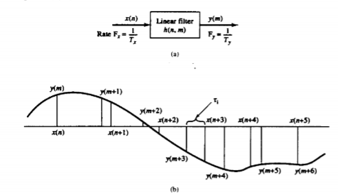
Fig 8 Sampling Rate Conversion
Decimation
Decimation, or down-sampling, consists of reducing the sampling rate by a factor M, cf. Figure 2.1. Here, the output is defined as
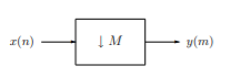
Fig 9 Decimation by factor M
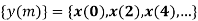
y(m) = x(mM)
i.e., it consists of every Mth element of the input signal. It is clear that the decimated signal y does not in general contain all information about the original signal x. Therefore, decimation is usually applied in filter banks and preceded by filters which extract the relevant frequency bands.
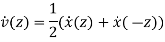
In order to analyze the frequency domain characteristics of a multirate processing system with decimation, we need to study the relation between the Fourier transforms, or the z-transforms, of the signals x and y. For simplicity we consider the case M = 2 only. Then the decimated signal y is given by
y(m) = x(2m)
 given the z-transforms of

z-transform of y(m) is given by


For finding the z-transform of y decimation is done in two stages as shown below

The above signal has z-transform as


The Fourier transform of the decimated signal y(m) is related to z-transform by
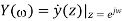
But 
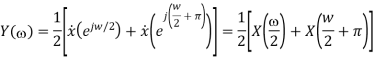
Where X is the Fourier-transform of the sequence {x(n)}. But from the properties of the Fourier transform (periodicity and symmetry) it follows that X(ω/2 + π) = X(ω/2 − π) = X(π − ω/2)∗ . Hence
The Fourier-transform of {y(m)} thus cannot distinguish between the frequencies ω/2 and π − ω/2 of {x(n)}. This is equivalent to the frequency folding phenomenon occurring when sampling a continuous-time signal. Hence, whereas the signal {x(n)} consists of frequencies in [0, π], the frequency contents of the decimated signal {y(m)} are restricted to the range [0, π/2]. Moreover, after decimation of the signal {x(n)}, its frequency components in [0, π/2] cannot be distinguished from the frequency components in the range [π/2, π].
Interpolation
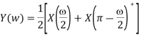
Expansion, or up-sampling, consists of increasing the sampling rate by a factor L, cf. Figure below. Here, the output is obtained by inserting L-1 zeros between successive values of the input x(n)
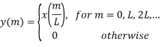
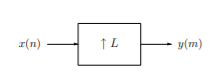
Fig 10 Interpolation by factor L
The expansion operation followed by interpolation leads to a representation of the signal x at a sampling rate increased by the factor L. The expanded signal {y(m)} has the z-transform

The Fourier Transform is

The transform Y (ω) at a given frequency ω ∈ [0, π] is thus equal to X(ωL), where ωL ∈ [0, Lπ]. But as the Fourier-transform is periodic with period 2π, we have X(ωL) = X(ωL + 2πk) = X((ω + 2πk L )L), and it follows that Y (ω) = Y (ω + 2πk L ). Hence Y (ω) is periodic, with L repetitions of X(ω) in the frequency range [0, 2π]. For example, for L = 2, we have X(2ω) = X(2ω − 2π) = X(2π − 2ω) ∗ = X(2(π − ω))∗ . Hence, for L = 2,
And Y (ω) is therefore uniquely defined by its values in the frequency band [0, π/2]. In order to reconstruct the correct interpolating signal at the higher sampling rate, an interpolating filter has to be introduced after the expansion. This is equivalent to the situation in D/A conversion, where a low-pass filter is used after the hold function.
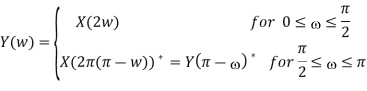
Analysis of Filter Banks
A basic operation in multirate signal processing is to decompose a signal into a number of sub band components, which can be processed at a lower rate corresponding to the bandwidth of the frequency bands. The down-sampling equation above shows that the down sampling mixes frequency components in the original signal by aliasing and frequency folding. Therefore, the signal should be filtered before decimation. Figure below shows the decomposition of a signal into two sub band components. The purpose of the filters H1 and H2 is to extract the low- and high-frequency components of the signal x before decimation. For example, the component xD1 may contain the low-frequency components of x, and the component xD2 may contain the low-frequency components of x. The set of filters shown in Figure below is called an analysis filter bank.
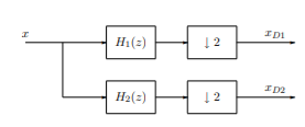
Fig 11 Single Decomposition into sub band component
If required, the signals may be decimated further into narrower sub-band components, Figure below. If H1 is a low-pass filter and H2 a high-pass filter, xD1 is the low-frequency component consisting of the sub-band [0, π/2], whereas xD21 and xD22 contain the sub-bands [π/2, 3π/4] and [3π/4, π], respectively. Notice that if possible, a convenient way to implement the decimation is to use stages with the decimation factor M = 2 as shown in Figure below. Then only one lowpass and one high-pass filter is required. For M > 2, bandpass filters with different passbands are required as well. After processing of the separate sub-band components, they are combined to reconstruct (a properly processed version of) the original signal at the original, higher sampling rate.
Fig 12 Filter Bank for Signal Decomposition
Therefore, the expanded signals should be filtered in order to extract the correct frequency components. The set of filters used to reconstruct the desired signal is called synthesis filter bank. Obviously, the analysis and synthesis filter banks form important parts of multirate signal processing systems with subband processing. The incoming signal is first decomposed by an analysis filter bank, and the outgoing signal is constructed using a synthesis filter bank,as shown in figure below
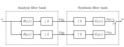
Fig 13: Multi-rate signal processing system with analysis and synthesis filter banks
Key takeaway
The set of filters used to reconstruct the desired signal is called synthesis filter bank.
References:
- S. K. Mitra, “Digital Signal Processing: A computer based approach”, McGraw Hill, 2011
- A.V. Oppenheim and R. W. Schafer, “Discrete Time Signal Processing”, Prentice Hall, 1989.
- J. G. Proakis and D.G. Manolakis, “Digital Signal Processing: Principles, Algorithms And Applications”, Prentice Hall, 1997.
- L. R. Rabiner and B. Gold, “Theory and Application of Digital Signal Processing”, Prentice Hall, 1992.
- J. R. Johnson, “Introduction to Digital Signal Processing”, Prentice Hall, 1992.
- Topic 14 Non-Parametric Spectral Density Estimation by H.J. Newton.


